Matching the WEST ICRH Antenna

In this notebook we investigate the various method to match a WEST ICRH antenna. By matching the antenna we mean to find 4 capacitances values \(C_1\), \(C_2\), \(C_3\) and \(C_4\) in order for the antenna to be operated at a given frequency \(f_0\).

%load_ext autoreload
%autoreload 2

import matplotlib.pyplot as plt
import skrf as rf
import numpy as np
import sys
from tqdm.notebook import tqdm

sys.path.append('..')
from west_ic_antenna import WestIcrhAntenna

rf.stylely()

from west_ic_antenna import WestIcrhAntenna

Matching Each Sides Separately

Here, each side of the antenna is matched separatly, which leads to two set of capacitances \((C_1, C_2)\) and \((C_3,C_4)\).

In the following example, both sides of the antenna are matched at the frequency \(f_0\), keeping opposite side unmatched (C=150pF):

f0 = 55.5e6
freq = rf.Frequency(54.5, 56.5, npoints=1001, unit='MHz')
ant = WestIcrhAntenna(frequency=freq)  # default is vacuum coupling

C_match_left = ant.match_one_side(f_match=f0, side='left', solution_number=1)
C_match_right = ant.match_one_side(f_match=f0, side='right', solution_number=1)
print('Left side matching point: ', C_match_left)
print('Right side matching point: ', C_match_right)

Wrong solution found ! Re-doing...
False solution #1: [150. 150.]
Wrong solution found ! Re-doing...
False solution #1: [150. 150.]
True solution #1: [49.96759702 47.93907498]
True solution #1: [49.73848258 48.10011086]
Left side matching point:  [np.float64(49.96759702378138), np.float64(47.93907498142962), 150, 150]
Right side matching point:  [150, 150, np.float64(49.73848258028963), np.float64(48.10011085922379)]

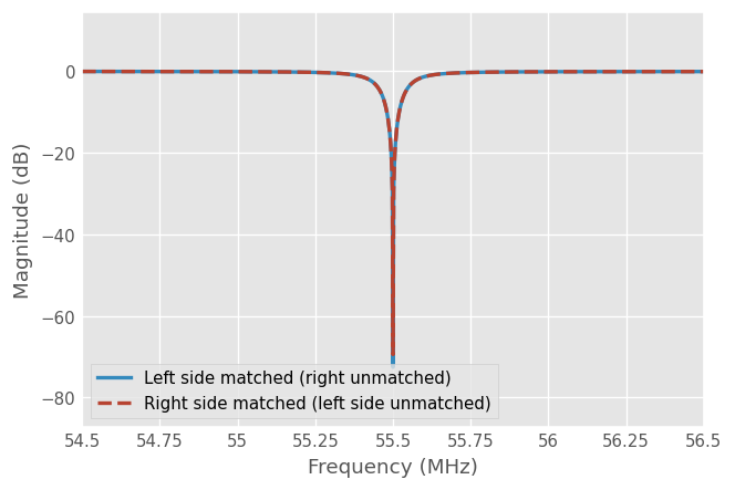
Let’s have a look to the RF reflection coefficient of each sides:

fig, ax = plt.subplots()
ant.circuit(Cs=C_match_left).network.plot_s_db(m=0, n=0, lw=2, ax=ax)
ant.circuit(Cs=C_match_right).network.plot_s_db(m=1, n=1, lw=2, ls='--', ax=ax)
ax.legend(('Left side matched (right unmatched)',
           'Right side matched (left side unmatched)'))

<matplotlib.legend.Legend at 0x7ec35aea9c40>

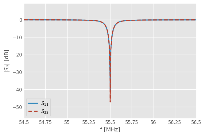
In reality, the precision at which one can tune the capacitance is not better than 1/100 pF, so one have to consider rounding optimal solutions to such precision :

C_match_left = ant.match_one_side(f_match=f0, side='left', solution_number=1, decimals=2)
C_match_right = ant.match_one_side(f_match=f0, side='right', solution_number=1, decimals=2)
print('Left side matching point: ', C_match_left)
print('Right side matching point: ', C_match_right)

True solution #1: [49.96759848 47.93907416]
Rounded result: [np.float64(49.97), np.float64(47.94), np.float64(150.0), np.float64(150.0)]
Wrong solution found ! Re-doing...
False solution #1: [150. 150.]
Wrong solution found ! Re-doing...
False solution #1: [150. 150.]
Wrong solution found ! Re-doing...
False solution #1: [150. 150.]
True solution #1: [49.73848104 48.10011184]
Rounded result: [np.float64(150.0), np.float64(150.0), np.float64(49.74), np.float64(48.1)]
Left side matching point:  [np.float64(49.97), np.float64(47.94), np.float64(150.0), np.float64(150.0)]
Right side matching point:  [np.float64(150.0), np.float64(150.0), np.float64(49.74), np.float64(48.1)]

Note that the performances are slightly degraded, but, it’s real life!

fig, ax = plt.subplots()
ant.circuit(Cs=C_match_left).network.plot_s_db(m=0, n=0, lw=2, ax=ax)
ant.circuit(Cs=C_match_right).network.plot_s_db(m=1, n=1, lw=2, ls='--', ax=ax)
ax.legend(('Left side matched (right unmatched)',
           'Right side matched (left side unmatched)'))
ax.set_ylabel('$|S_{ii}|$ [dB]')
ax.set_xlabel('f [MHz]')
ax.legend(('$S_{11}$', '$S_{22}$'))

<matplotlib.legend.Legend at 0x7ec35aea5d90>

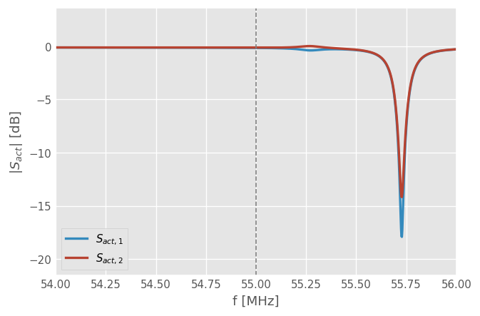
Frequency Shift for Dipole Excitation

The coupling between antenna’s sides requires shifting the frequency with respect to the matching frequency used for each side separately.

Thus, if the optimal capacitor set for both side are of the same kind (i.e. either both C_top>C_bot or both C_top<C_bot), then dipole excitation (phase \((0,\pi)\)) requires to shift the frequency to higher frequency to operate the antenna in a optimal conditions:

# dipole excitation
power = [1, 1]
phase = [0, rf.pi]
# combine both separate solutions
C_match = [C_match_left[0], C_match_left[1], C_match_right[2], C_match_right[3]]
# looking to the active s parameters:
s_act = ant.s_act(power, phase, Cs=C_match)
# finding the optimum frequency
idx_f_opt = np.argmin(np.abs(s_act[:,0]))
f_opt = freq.f[idx_f_opt]
delta_f = f_opt - f0
print(f'Optimum frequency is f_opt={f_opt/1e6} MHz --> {delta_f/1e6} MHz shift' )

Optimum frequency is f_opt=55.728 MHz --> 0.228 MHz shift

/tmp/ipykernel_3150/3939305869.py:3: FutureWarning: skrf.pi is deprecated. Please import pi from skrf.tlineFunctions instead.
  phase = [0, rf.pi]

fig, ax = plt.subplots()
ax.plot(freq.f_scaled, 20*np.log10(np.abs(s_act)), lw=2)
ax.axvline(f0/1e6, ls='--', color='gray')
ax.axvline(f_opt/1e6, ls='--', color='k')
ax.set_ylabel('$|S_{act}|$ [dB]')
ax.set_xlabel('f [MHz]')
ax.legend(('$S_{act,1}$', '$S_{act,2}$'))
ax.set_title('Dipole excitation')

Text(0.5, 1.0, 'Dipole excitation')

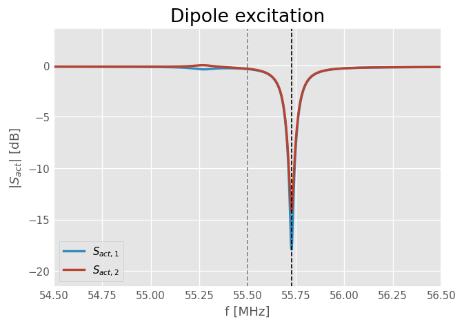
However, the reflection coefficient is not that low (-15 to -20 dB at best). That means that there is certainly a sweeter spot of the capacitor set.

C_opt = ant.match_both_sides(f_match=55.728e6, decimals=2)
print(C_opt)

Looking for individual solutions separately for 1st guess...
Wrong solution found ! Re-doing...
False solution #1: [150. 150.]
Wrong solution found ! Re-doing...
False solution #1: [150. 150.]
True solution #1: [49.30690696 47.3182471 ]
Rounded result: [np.float64(49.31), np.float64(47.32), np.float64(150.0), np.float64(150.0)]
True solution #1: [49.0796221  47.47779491]
Rounded result: [np.float64(150.0), np.float64(150.0), np.float64(49.08), np.float64(47.48)]
Searching for the active match point solution...
Reducing search range to +/- 5pF around individual solutions
True solution #1: [49.87570009 48.04905491 49.55474717 48.25485594]
Rounded result: [np.float64(49.88), np.float64(48.05), np.float64(49.55), np.float64(48.25)]
[np.float64(49.88), np.float64(48.05), np.float64(49.55), np.float64(48.25)]

The difference is:

np.array(C_opt) - np.array(C_match)

array([-0.09,  0.11, -0.19,  0.15])

That is, one should:

• decrease slightly the top capacitors

• increase slightly the bottom capacitors

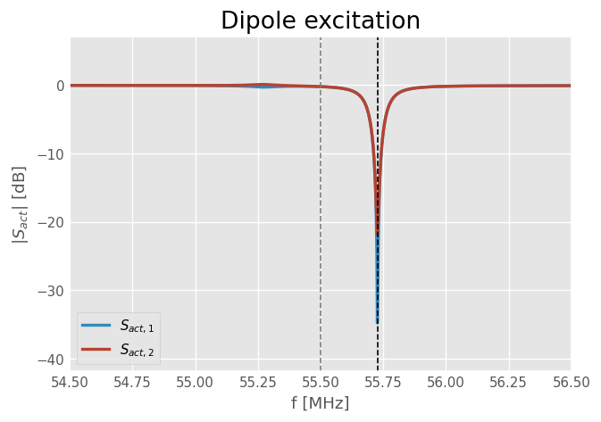
As a rule of thumb, at 55.5 MHz, we can remember to do -0.1pF for top and +0.1pF for bottom capacitors. Doing, so, we get a better match point (between -20 and -30 dB)

C_match_improved = [C_match[0] - 0.1,
                    C_match[1] + 0.1,
                    C_match[2] - 0.1,
                    C_match[3] + 0.1]
fig, ax = plt.subplots()
ax.plot(freq.f_scaled, ant.s_act_db(Cs=C_match_improved, power=[1,1], phase=[0,np.pi]), lw=2)
ax.axvline(f0/1e6, ls='--', color='gray')
ax.axvline(f_opt/1e6, ls='--', color='k')
ax.set_ylabel('$|S_{act}|$ [dB]')
ax.set_xlabel('f [MHz]')
ax.legend(('$S_{act,1}$', '$S_{act,2}$'))
ax.set_title('Dipole excitation')

/home/docs/checkouts/readthedocs.org/user_builds/west-ic-antenna/checkouts/latest/doc/../west_ic_antenna/antenna.py:1316: FutureWarning: skrf.mag_2_db is deprecated. Please import mag_2_db from skrf.mathFunctions instead.
  return rf.mag_2_db(np.abs(self.s_act(power, phase, Cs)))

Text(0.5, 1.0, 'Dipole excitation')

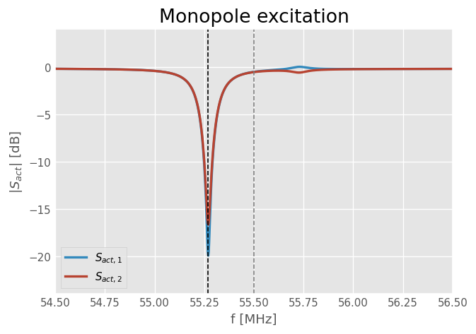
Monopole excitation (phase \((0,0)\)) at the contrary requires shifting the operating frequency toward lower frequencies:

# monopole excitation
power = [1, 1]
phase = [0, 0]
# combine both separate solutions
C_match = [C_match_left[0], C_match_left[1], C_match_right[2], C_match_right[3]]
# looking to the active s parameters:
s_act = ant.s_act(power, phase, Cs=C_match)
# finding the optimum frequency
idx_f_opt = np.argmin(np.abs(s_act[:,0]))
f_opt = freq.f[idx_f_opt]
delta_f = f_opt - f0
print(f'Optimum frequency is f_opt={f_opt/1e6} MHz --> {delta_f/1e6} MHz shift' )

Optimum frequency is f_opt=55.27 MHz --> -0.23 MHz shift

fig, ax = plt.subplots()
ax.plot(freq.f_scaled, 20*np.log10(np.abs(s_act)), lw=2)
ax.axvline(f0/1e6, ls='--', color='gray')
ax.axvline(f_opt/1e6, ls='--', color='k')
ax.set_ylabel('$|S_{act}|$ [dB]')
ax.set_xlabel('f [MHz]')
ax.legend(('$S_{act,1}$', '$S_{act,2}$'))
ax.set_title('Monopole excitation')

Text(0.5, 1.0, 'Monopole excitation')

The matching can also be improved:

C_opt_mono = ant.match_both_sides(f_match=55.27e6, decimals=2, power=[1,1], phase=[0,0])
print(C_opt_mono)

Looking for individual solutions separately for 1st guess...
Wrong solution found ! Re-doing...
False solution #1: [150. 150.]
True solution #1: [50.64166802 48.57244536]
Rounded result: [np.float64(50.64), np.float64(48.57), np.float64(150.0), np.float64(150.0)]
Wrong solution found ! Re-doing...
False solution #1: [150. 150.]
True solution #1: [50.4106761  48.73500668]
Rounded result: [np.float64(150.0), np.float64(150.0), np.float64(50.41), np.float64(48.74)]
Searching for the active match point solution...
Reducing search range to +/- 5pF around individual solutions
True solution #1: [50.06506866 47.82371195 49.88914693 47.9801329 ]
Rounded result: [np.float64(50.07), np.float64(47.82), np.float64(49.89), np.float64(47.98)]
[np.float64(50.07), np.float64(47.82), np.float64(49.89), np.float64(47.98)]

So a difference of:

np.array(C_opt_mono) - np.array(C_match)

array([ 0.1 , -0.12,  0.15, -0.12])

That is the opposite trend than for dipole:

• increase slightly top capacitors (~ +0.1 pF as a rule of thumb)

• decrease slightly bot capacitors (~ -0.1 pF as a rule of thumb)

Matching Both Sides at the same time

It is also possible to optimize the antenna directly for the target frequency and for a given excitation. Matching both sides at the same time in fact matches each side separately, then find the optimum points using these solutions as starting point to help the convergence of the optimization.

Two methods are available to match both sides of the antenna: match_both_sides which use the NumPy optimisation routines, and match_both_sides_iterative which uses the feedback matching algorithm (see matching_automatic.ipynb for more details). The primer is more robust in finding a solution, eventually at the price of a longer calculation. The later method can indeed be “lost” if the ideal solution is not close enough (or if the optimal region is too narrow, like under vacuum).

f0 = 55e6
freq = rf.Frequency(54, 56, npoints=1001, unit='MHz')
ant = WestIcrhAntenna(frequency=freq)  # default is vacuum coupling

# antenna excitation to match for
power = [1, 1]  # W
phase = [0, np.pi]  # dipole

ant.DEBUG=True  # display additional messages
# Providing an initial guess C0 skip the search on both sides separately
C0 = [C_match_left[0], C_match_left[1], C_match_right[2], C_match_right[3]]
C_opt_vacuum_dipole = ant.match_both_sides(f_match=f0, power=power, phase=phase, C0=C0, decimals=2)

Using given first guess: [np.float64(49.97), np.float64(47.94), np.float64(49.74), np.float64(48.1)]
Searching for the active match point solution...
Reducing search range to +/- 5pF around individual solutions
[49.97 47.94 49.74 48.1 ] 1.391286194413165
[49.97000001 47.94       49.74       48.1       ] 1.391286194360197
[49.97       47.94000001 49.74       48.1       ] 1.3912861944307828
[49.97       47.94       49.74000001 48.1       ] 1.3912861943843553
[49.97       47.94       49.74       48.10000001] 1.3912861944232966
Optimization terminated successfully    (Exit mode 0)
            Current function value: 1.391286194413165
            Iterations: 1
            Function evaluations: 5
            Gradient evaluations: 1
True solution #1: [49.97 47.94 49.74 48.1 ]
Rounded result: [np.float64(49.97), np.float64(47.94), np.float64(49.74), np.float64(48.1)]

f0 = 55e6
freq = rf.Frequency(54, 56, npoints=1001, unit='MHz')
ant = WestIcrhAntenna(frequency=freq)  # default is vacuum coupling

# looking to the active s parameters:
s_act = ant.s_act(power, phase, Cs=C_opt_vacuum_dipole)

fig, ax = plt.subplots()
ax.plot(freq.f_scaled, 20*np.log10(np.abs(s_act)), lw=2)
ax.axvline(f0/1e6, ls='--', color='gray')
ax.set_ylabel('$|S_{act}|$ [dB]')
ax.set_xlabel('f [MHz]')
ax.legend(('$S_{act,1}$', '$S_{act,2}$'))

<matplotlib.legend.Legend at 0x7ec3612c1be0>

Manual Matching on Plasma

When the antenna is facing the plasma, the coupling resistance increases and the antenna matching is affected.

If the operator keeps the matchpoint obtained on vacuum (in dipole for example), the antenna will have the following behaviour:

# changing the front-face of the antenna to a plasma case
freq = rf.Frequency(54, 56, npoints=1001, unit='MHz')
front_face_plasma = WestIcrhAntenna.interpolate_front_face(Rc=1, source='TOPICA-L-mode')
ant = WestIcrhAntenna(frequency=freq, front_face=front_face_plasma)

# looking to the active s parameters in dipole:
powers = [1 ,1]
phases = [0, np.pi]
s_act = ant.s_act(powers, phases , Cs=C_opt_vacuum_dipole)

fig, ax = plt.subplots()
ax.plot(freq.f_scaled, 20*np.log10(np.abs(s_act)), lw=2)
ax.axvline(f0/1e6, ls='--', color='gray')
ax.set_ylabel('$|S_{act}|$ [dB]')
ax.set_xlabel('f [MHz]')
ax.legend(('$S_{act,1}$', '$S_{act,2}$'))
ax.set_title('Reflection on plasma using vacuum matching setpoint')

Text(0.5, 1.0, 'Reflection on plasma using vacuum matching setpoint')

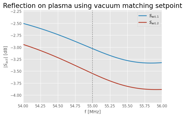
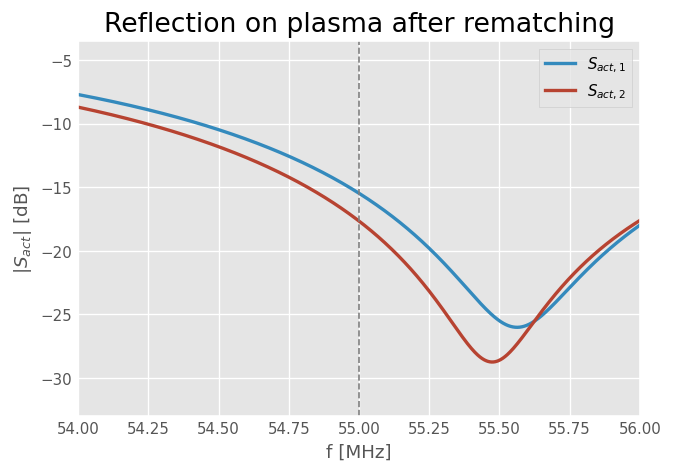
Thus, it is necessary to re-adapt the capacitors to improve the matching of the antenna on plasma:

C_match_plasma = ant.match_both_sides(f0, power=powers, phase=phases, C0=C_opt_vacuum_dipole)

Using given first guess: [np.float64(49.97), np.float64(47.94), np.float64(49.74), np.float64(48.1)]
Searching for the active match point solution...
Reducing search range to +/- 5pF around individual solutions
True solution #1: [54.1244474  45.89265233 53.7219561  45.92680806]

s_act = ant.s_act(powers, phases , Cs=C_match_plasma)

fig, ax = plt.subplots()
ax.plot(freq.f_scaled, 20*np.log10(np.abs(s_act)), lw=2)
ax.axvline(f0/1e6, ls='--', color='gray')
ax.set_ylabel('$|S_{act}|$ [dB]')
ax.set_xlabel('f [MHz]')
ax.legend(('$S_{act,1}$', '$S_{act,2}$'))
ax.set_title('Reflection on plasma after rematching')

Text(0.5, 1.0, 'Reflection on plasma after rematching')

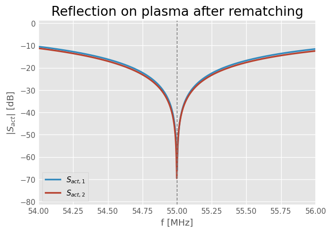
If we compare the differences between capacitances setpoint between vacuum and plasma cases, we see that the difference between the values go like this:

• top capacitances are increased

• bottom capacitances are decreased

Thus, the “distance” between top and bottom capacitance is increased.

np.array(C_match_plasma) - np.array(C_opt_vacuum_dipole)

array([ 4.1544474 , -2.04734767,  3.9819561 , -2.17319194])

The capacitance shift to apply with respect to the vacuum setpoint depends of the coupling resistance of the plasma.

We can use this property to deduce the set of capacitors to use during plasma operation. Below we generate a series of various plasma loading cases, of increasing coupling resistance \(R_c\). For each case we search for and we store the setpoints.

C_matchs = []

# note: on plasma loads, the iterative method is faster
# important : increase the gap between capacitances start point for the algorith to converge for high Rc cases
C0 = np.array(C_opt_vacuum_dipole) + np.array([+5, -5, +5, -5])

Rcs1 = np.linspace(0.39, 1.7, 10)  # TOPICA "H-mode" (low coupling)
for Rc in tqdm(Rcs1):
    _plasma = WestIcrhAntenna.interpolate_front_face(Rc=Rc, source='TOPICA-H-mode')
    _ant = WestIcrhAntenna(frequency=freq, front_face=_plasma)
    _C_match = _ant.match_both_sides_iterative(f0, power=powers, phase=phases, Cs=C_opt_vacuum_dipole)
    C_matchs.append(_C_match)


Rcs2 = np.linspace(1, 2.9, 10)  # TOPICA "L-mode" (higher coupling)
for Rc in tqdm(Rcs2):
    _plasma = WestIcrhAntenna.interpolate_front_face(Rc=Rc, source='TOPICA-L-mode')
    _ant = WestIcrhAntenna(frequency=freq, front_face=_plasma)
    _C_match = _ant.match_both_sides_iterative(f0, power=powers, phase=phases, Cs=C0)
    C_matchs.append(_C_match)

Stopped after 9 iterations
Solution found: [np.float64(52.59447260295835), np.float64(47.255722561972945), np.float64(52.32814575537496), np.float64(47.44211425794061)]
Stopped after 13 iterations
Solution found: [np.float64(53.22738503611959), np.float64(47.080910472129304), np.float64(52.94954515949542), np.float64(47.258540892085435)]
Stopped after 16 iterations
Solution found: [np.float64(53.79184124688131), np.float64(46.96216161158988), np.float64(53.50732252911463), np.float64(47.13466139754257)]
Stopped after 20 iterations
Solution found: [np.float64(54.30267375096152), np.float64(46.87089989980136), np.float64(54.01299457693531), np.float64(47.03996062781131)]
Stopped after 25 iterations
Solution found: [np.float64(54.767644814979576), np.float64(46.79672437989013), np.float64(54.472353841030355), np.float64(46.96299242316423)]
Stopped after 31 iterations
Solution found: [np.float64(55.19269634061181), np.float64(46.73451589267797), np.float64(54.89085293705217), np.float64(46.897678737308276)]
Stopped after 37 iterations
Solution found: [np.float64(55.57920491127813), np.float64(46.68899173153471), np.float64(55.272997650713805), np.float64(46.85072222286625)]
Stopped after 46 iterations
Solution found: [np.float64(55.92604587940951), np.float64(46.64009766028608), np.float64(55.61497168712195), np.float64(46.79985441197666)]
Stopped after 47 iterations
Solution found: [np.float64(55.67387678069811), np.float64(47.19280525943693), np.float64(-22.103810713638843), np.float64(47.63062872958513)]
Stopped after 61 iterations
Solution found: [np.float64(56.3681111490302), np.float64(47.46651279331395), np.float64(-70.60006214415972), np.float64(47.87909804678935)]

Stopped after 22 iterations
Solution found: [np.float64(53.94003228625973), np.float64(45.94768654622772), np.float64(53.521571590490645), np.float64(45.98388148494275)]
Stopped after 24 iterations
Solution found: [np.float64(54.24471829895416), np.float64(45.82677433380006), np.float64(53.82697444390541), np.float64(45.8439304742466)]
Stopped after 27 iterations
Solution found: [np.float64(54.548837652114806), np.float64(45.67783804514688), np.float64(54.13154120890661), np.float64(45.662497742454676)]
Stopped after 29 iterations
Solution found: [np.float64(54.83439824939769), np.float64(45.539349013495), np.float64(54.4200794397674), np.float64(45.48655083117148)]
Stopped after 30 iterations
Solution found: [np.float64(55.06323124838135), np.float64(45.40878875023448), np.float64(54.65495429013614), np.float64(45.31484343848153)]
Stopped after 31 iterations
Solution found: [np.float64(55.096917719265676), np.float64(45.17855349033404), np.float64(54.67970446567908), np.float64(44.975121552050766)]
Stopped after 35 iterations
Solution found: [np.float64(54.85980910385082), np.float64(44.80901753738203), np.float64(54.389622657453835), np.float64(44.32327434019762)]
Stopped after 48 iterations
Solution found: [np.float64(54.546973527324226), np.float64(44.252222672653545), np.float64(54.0001594544397), np.float64(43.169593653404064)]
Stopped after 54 iterations
Solution found: [np.float64(53.81427501341985), np.float64(43.05065471816488), np.float64(51.80585825428513), np.float64(37.588537940391696)]
Stopped after 61 iterations
Solution found: [np.float64(58.59916284009732), np.float64(47.577741789282044), np.float64(0.06229665309216048), np.float64(48.58630957932011)]

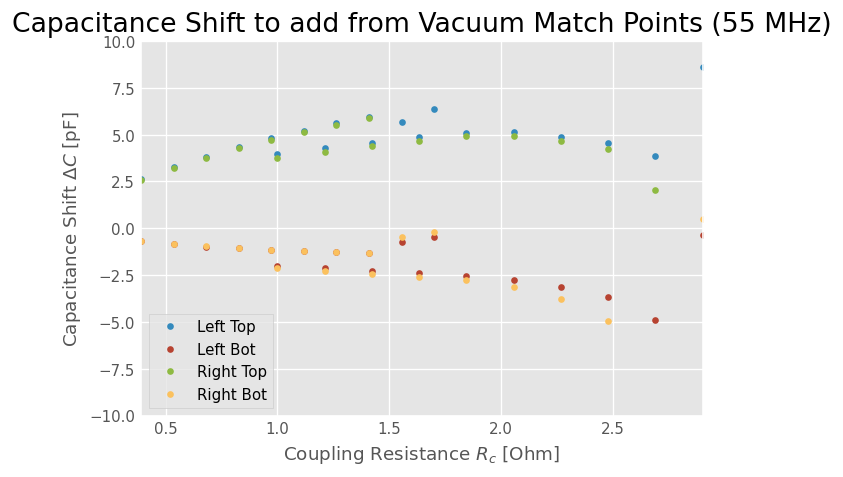
Let’s plot the average capacitance shift to apply versus the coupling resistance of the plasma loading scenario:

Rcs3 = np.linspace(0.3, 1.6, 10)

diff_C = np.array(C_matchs) - np.array(C_opt_vacuum_dipole)

Rcs = np.concatenate([Rcs1, Rcs2])
fig, ax = plt.subplots()
ax.plot(Rcs, diff_C, 'o')
ax.set_xlabel('Coupling Resistance $R_c$ [Ohm]')
ax.set_ylabel('Capacitance Shift $\Delta C$ [pF]')
ax.set_title('Capacitance Shift to add from Vacuum Match Points (55 MHz)')
ax.legend(['Left Top', 'Left Bot', 'Right Top', 'Right Bot'])
ax.set_ylim(-10, 10)

<>:5: SyntaxWarning: invalid escape sequence '\D'
<>:5: SyntaxWarning: invalid escape sequence '\D'
/tmp/ipykernel_3150/668917840.py:5: SyntaxWarning: invalid escape sequence '\D'
  ax.set_ylabel('Capacitance Shift $\Delta C$ [pF]')

(-10.0, 10.0)

Automatic Matching

Here is just a glimpse of the automatic matching capabilities. You will find more on automatic matching in the automatic matching section

Let’s assume we start from a non-optimal situation, that is we enlarge the capacitance differences from a vacuum matching from a rather arbitrary value:

Cs = list(np.array(C_opt_vacuum_dipole) + np.array([+3, -3, +3, -3]))

Then, using the capacitor predictor, we calculate the capacitance set to reach:

# Evaluate this cell a few times to see the convergence to the optimal matching
C_left, C_right, err = ant.capacitor_predictor(powers, phases, Cs=Cs)
idx_f = np.argmin(np.abs(ant.frequency.f - 55e6))
Cs = [*C_left[idx_f], *C_right[idx_f]]

print(Cs)

[np.float64(53.29701374291504), np.float64(44.909009129936784), np.float64(52.98851438651536), np.float64(45.0811052070515)]

s_act = ant.s_act(powers, phases , Cs=Cs)

fig, ax = plt.subplots()
ax.plot(freq.f_scaled, 20*np.log10(np.abs(s_act)), lw=2)
ax.axvline(f0/1e6, ls='--', color='gray')
ax.set_ylabel('$|S_{act}|$ [dB]')
ax.set_xlabel('f [MHz]')
ax.legend(('$S_{act,1}$', '$S_{act,2}$'))
ax.set_title('Reflection on plasma after rematching')

Text(0.5, 1.0, 'Reflection on plasma after rematching')

This plot should be benchmarked against plasma measurements.

from IPython.core.display import HTML
def _set_css_style(css_file_path):
    """
    Read the custom CSS file and load it into Jupyter
    Pass the file path to the CSS file
    """
    styles = open(css_file_path, "r").read()
    s = '<style>%s</style>' % styles
    return HTML(s)

_set_css_style('custom.css')