Automatic Matching
This notebooks explains how the automatic matching is implemented on WEST ICRH antenna.
[1]:
%load_ext autoreload
%autoreload 2
[2]:
import matplotlib.pyplot as plt
import skrf as rf
import numpy as np
import sys
from tqdm.notebook import tqdm

sys.path.append('..')
from west_ic_antenna import WestIcrhAntenna
Introduction
The WEST automatic matching of the capacitors of an ICRH antenna is made with a negative feedback loop. ICRH Operator defines the desired input impedance at the T-junction setpoint \(Z_{T,SP}\). This setpoint is compared to the actual impedance at the T-junction \(Z_T\) and capacitors are adjusted to minimize this difference in realtime. The input impedance at the T-junction is determined from the input impedance at the bidirective coupler located behind the antennas.
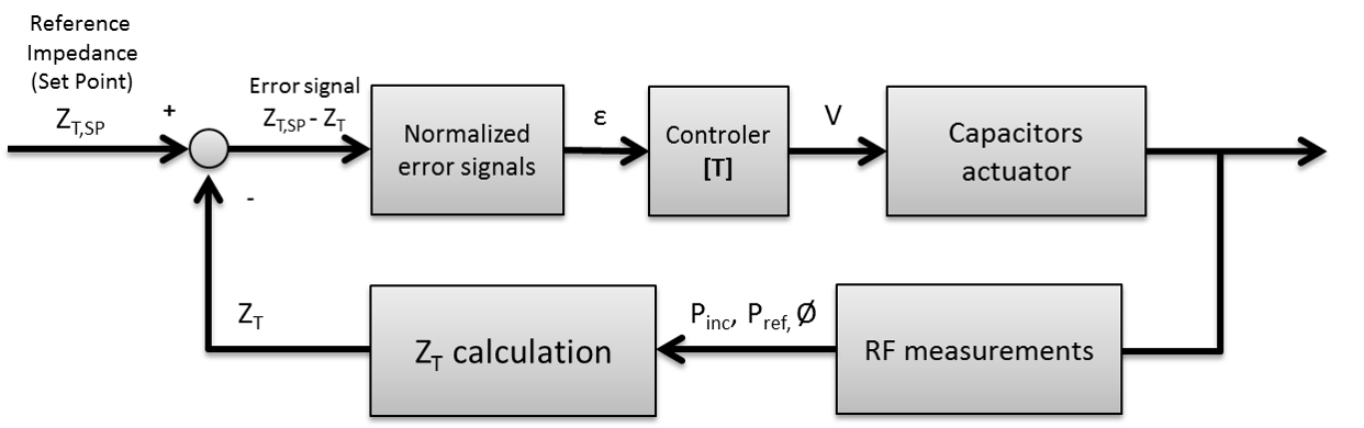
The different steps are described below:
RF Measurements: the forward \(P_{fwd}\) and reflected powers \(P_{ref}\) are measured at the bidirective coupler located behind an antenna. The phase difference between these two \(\Phi_\Gamma\) is also measured. The impedance at the bidirective coupler \(Z_{coupler}\) is deduced from the complex reflection coefficient \(\Gamma\) :
where \(Z_0\)=30 Ω is the characteristic impedance of the transmission line and \(\Phi_c\) a possible phase correction that the IC operator can tune.
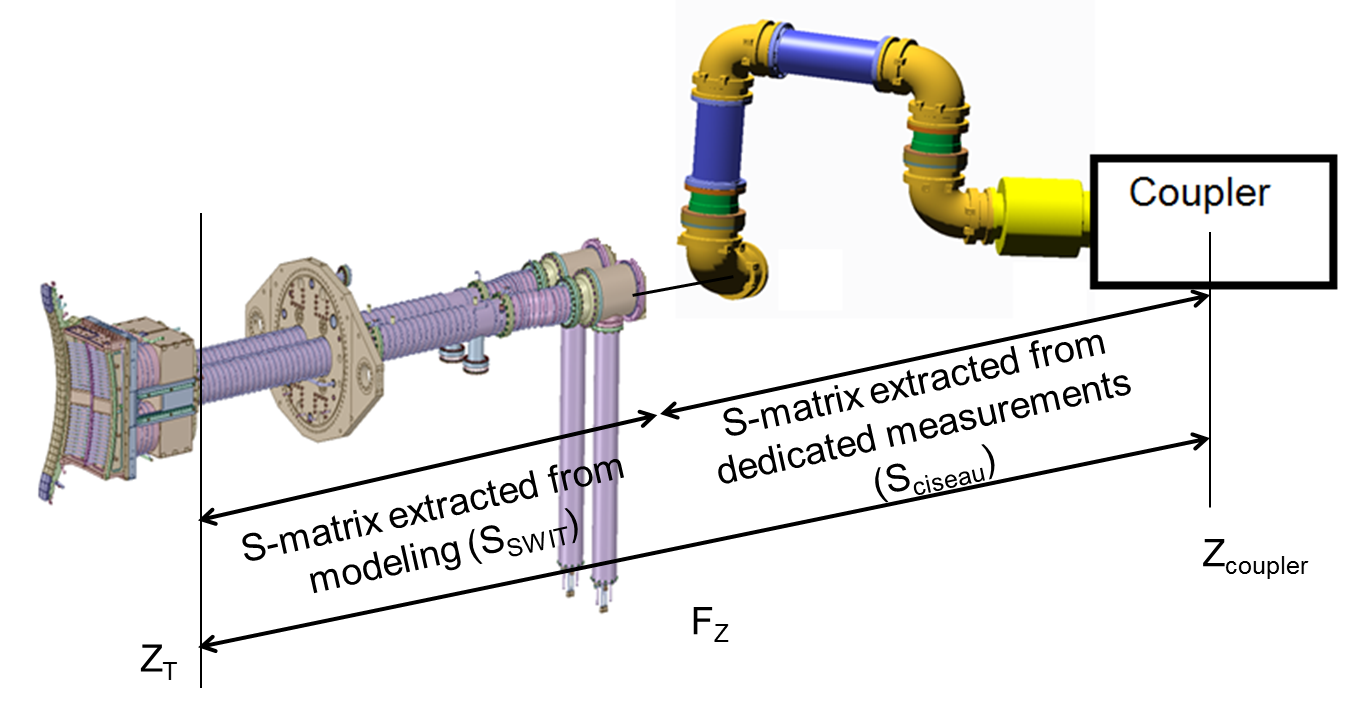
\(Z_T\) Calculation:
Let \(A\) the ABCD matrix of the assembly of the piece of transmission line between the bidirective coupler and the antenna elements up to the T-junction. This matrix has been deduced from the CAD model of the antenna (\(S_{SWIT}\)) and from the measurement of the piece of transmission lines (\(S_{ciseau}\)) for each antennas (which can differ in length).
The impedance at the T-junction is deduced from the impedance \(Z_{coupler}\) (here asssuming port 1 is located at the T junction):
NB: if port 1 is instead the 30 Ohm side, the equation would have been:
Normalized error signal: the relative change of the measured error \(\varepsilon\) is :
Controller: gives a velocity request \(V_r=(V_{r,top}, V_{r,bot})\) to the capacitors actuator:
The derivation of the matrix \(\mathbf{T}\) is detailed in the next section
Controler Development
Introduction
The impedance at the T-junction \(Z_T\) is a function of the capacitances set \(\mathbf{C}=( C_{top}, C_{bot})^t\):
Close to the desired capacitances solution \(\mathbf{C}_{SP}=(C_{top,SP}, C_{bot,SP})^t\), the previous equation can be approximated thanks to the Taylor theorem:
with
We define later \(\delta\mathbf{C}=\mathbf{C} - \mathbf{C}_{SP}\) and recalls that the first term on the right hand side \(Z_T(\mathbf{C}_{SP})\) corresponds to the desired Set Point \(Z_{T,SP}\).
Splitting \(Z_T\) into real and imaginary parts leads to:
where
The previous formula can be inversed to given the required \(\delta \mathbf{C}\) increment to reach the Set Point:
The goal of the this section is to determine the elements of the Jacobian matrix \(\mathbf{D}\).
Numerical Values of the Jacobian
Let’s define a WEST ICRH antenna for a given frequency:
[3]:
f0 = 55  # MHz
freq0 = rf.Frequency(f0, f0, unit='MHz', npoints=1)
antenna = WestIcrhAntenna(frequency=freq0,
                          front_face='../west_ic_antenna/data/Sparameters/front_faces/TOPICA/S_TSproto12_55MHz_Hmode_LAD6-2.5cm.s4p')
antenna.front_face_Rc()
[3]:
array([[1.60955001, 1.60955001]])
Now we calculate the ideal matching point (for an half side only):
[4]:
C_match = antenna.match_one_side(f_match=f0*1e6,
                                 side='left', solution_number=1)
print(C_match)
Wrong solution found ! Re-doing...
False solution #1: [150. 150.]
True solution #1: [53.75340284 46.49026767]
[np.float64(53.75340283922421), np.float64(46.490267667066604), 150, 150]
[5]:
power = [1,1e-6]
phase = [0,0]
Let’s calculate the derivate of \(Z_T\) around the match point:
[6]:
delta_C_tops = np.linspace(-10, 10, 51)
delta_C_bots = np.linspace(-10, 10, 51)
[7]:
# derivatives vs Ctop
z_Ts = []
z_T_SP = (2.9-0.3j)

for delta_C_top in delta_C_tops:
    # z_T
    _z_T = antenna.z_T(power, phase, Cs=[C_match[0]+delta_C_top, C_match[1], 150, 150])
    z_Ts.append(_z_T[:,0]) # left side
z_Ts = np.array(z_Ts).squeeze()
dz_Ts_dCtop = np.diff(z_Ts)

# normalized error and derivative
eps_Ctop = (z_T_SP - z_Ts)/z_Ts
deps_dCtop = np.diff(eps_Ctop)

# diff vs Cbot
z_Ts = []
for delta_C_bot in delta_C_bots:
    # z_T
    _z_T = antenna.z_T(power, phase, Cs=[C_match[0], C_match[1]+delta_C_bot, 150, 150])
    z_Ts.append(_z_T[:,0]) # left side
z_Ts = np.array(z_Ts).squeeze()/z_T_SP
dz_Ts_dCbot = np.diff(z_Ts)

# normalized error and derivative
eps_Cbot = (z_T_SP - z_Ts)/z_Ts
deps_dCbot = np.diff(eps_Cbot)
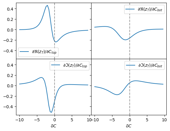
Below are the traces of the derivatives of \(Z_T\) around the Set Point:
[8]:
fig, axes = plt.subplots(2, 2, sharex=True, sharey=True)
axes[0,0].plot(delta_C_tops[:-1], dz_Ts_dCtop.real, label='$\partial \Re(z_T)/\partial C_{top}$')
axes[0,1].plot(delta_C_bots[:-1], dz_Ts_dCbot.real, label='$\partial \Re(z_T)/\partial C_{bot}$')
axes[1,0].plot(delta_C_tops[:-1], dz_Ts_dCtop.imag, label='$\partial \Im(z_T)/\partial C_{top}$')
axes[1,1].plot(delta_C_bots[:-1], dz_Ts_dCbot.imag, label='$\partial \Im(z_T)/\partial C_{bot}$')
axes[1,0].set_xlabel('$\delta C$')
axes[1,1].set_xlabel('$\delta C$')
[ax.legend() for ax in axes.ravel()]
[ax.axvline(0, color='gray', ls='--', alpha=0.8) for ax in axes.ravel()]
fig.subplots_adjust(wspace=0.0, hspace=0.0)
<>:2: SyntaxWarning: invalid escape sequence '\p'
<>:3: SyntaxWarning: invalid escape sequence '\p'
<>:4: SyntaxWarning: invalid escape sequence '\p'
<>:5: SyntaxWarning: invalid escape sequence '\p'
<>:6: SyntaxWarning: invalid escape sequence '\d'
<>:7: SyntaxWarning: invalid escape sequence '\d'
<>:2: SyntaxWarning: invalid escape sequence '\p'
<>:3: SyntaxWarning: invalid escape sequence '\p'
<>:4: SyntaxWarning: invalid escape sequence '\p'
<>:5: SyntaxWarning: invalid escape sequence '\p'
<>:6: SyntaxWarning: invalid escape sequence '\d'
<>:7: SyntaxWarning: invalid escape sequence '\d'
/tmp/ipykernel_2791/1404037713.py:2: SyntaxWarning: invalid escape sequence '\p'
  axes[0,0].plot(delta_C_tops[:-1], dz_Ts_dCtop.real, label='$\partial \Re(z_T)/\partial C_{top}$')
/tmp/ipykernel_2791/1404037713.py:3: SyntaxWarning: invalid escape sequence '\p'
  axes[0,1].plot(delta_C_bots[:-1], dz_Ts_dCbot.real, label='$\partial \Re(z_T)/\partial C_{bot}$')
/tmp/ipykernel_2791/1404037713.py:4: SyntaxWarning: invalid escape sequence '\p'
  axes[1,0].plot(delta_C_tops[:-1], dz_Ts_dCtop.imag, label='$\partial \Im(z_T)/\partial C_{top}$')
/tmp/ipykernel_2791/1404037713.py:5: SyntaxWarning: invalid escape sequence '\p'
  axes[1,1].plot(delta_C_bots[:-1], dz_Ts_dCbot.imag, label='$\partial \Im(z_T)/\partial C_{bot}$')
/tmp/ipykernel_2791/1404037713.py:6: SyntaxWarning: invalid escape sequence '\d'
  axes[1,0].set_xlabel('$\delta C$')
/tmp/ipykernel_2791/1404037713.py:7: SyntaxWarning: invalid escape sequence '\d'
  axes[1,1].set_xlabel('$\delta C$')
Below are the plot of the derivatives of the error signal \(\varepsilon\) around the Set Point:
[9]:
fig, axes = plt.subplots(2, 2, sharex=True, sharey=True)
axes[0,0].plot(delta_C_tops[:-1], deps_dCtop.real, label=r'$\partial \Re(\varepsilon)/\partial C_{top}$')
axes[0,1].plot(delta_C_bots[:-1], deps_dCbot.real, label=r'$\partial \Re(\varepsilon)/\partial C_{bot}$')
axes[1,0].plot(delta_C_tops[:-1], deps_dCtop.imag, label=r'$\partial \Im(\varepsilon)/\partial C_{top}$')
axes[1,1].plot(delta_C_bots[:-1], deps_dCbot.imag, label=r'$\partial \Im(\varepsilon)/\partial C_{bot}$')
axes[1,0].set_xlabel('$\delta C$')
axes[1,1].set_xlabel('$\delta C$')
[ax.legend() for ax in axes.ravel()]
[ax.axvline(0, color='gray', ls='--', alpha=0.8) for ax in axes.ravel()]
fig.subplots_adjust(wspace=0.0, hspace=0.0)
<>:6: SyntaxWarning: invalid escape sequence '\d'
<>:7: SyntaxWarning: invalid escape sequence '\d'
<>:6: SyntaxWarning: invalid escape sequence '\d'
<>:7: SyntaxWarning: invalid escape sequence '\d'
/tmp/ipykernel_2791/4209014612.py:6: SyntaxWarning: invalid escape sequence '\d'
  axes[1,0].set_xlabel('$\delta C$')
/tmp/ipykernel_2791/4209014612.py:7: SyntaxWarning: invalid escape sequence '\d'
  axes[1,1].set_xlabel('$\delta C$')
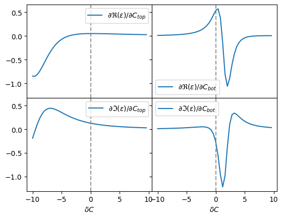
Below are the values of the derivative at the Set Point:
[10]:
idx = np.argmin(np.abs(delta_C_bots))
print('dz_T/dCtop:', dz_Ts_dCtop[idx])
print('dz_T/dCbot:', dz_Ts_dCbot[idx])

print('de/dCtop:', deps_dCtop[idx])
print('de/dCbot:', deps_dCbot[idx])
dz_T/dCtop: (-0.22004299686224504-0.312575045965821j)
dz_T/dCbot: (-0.1654958898292136+0.050739775866537086j)
de/dCtop: (0.05176663481297227+0.1282250392516446j)
de/dCbot: (0.5391833061406051-0.26410011247743803j)
As the \(\mathbf{D}\) matrix depends of the conditions (coupling, excitation), it is not possible to determine it exactly in advance in real experiments.
An approximative solution is to take only the sign of the derivatives: hence few iterations are needed until converging to the solution.
Note that this algorithm will diverge if the start point is not close enough from the optimal solution:
[11]:
D = np.array([[dz_Ts_dCtop[idx].real, dz_Ts_dCbot[idx].real],
              [dz_Ts_dCtop[idx].imag, dz_Ts_dCbot[idx].imag]])
print(np.sign(D))
[[-1. -1.]
 [-1.  1.]]
So, for solution 1, one would obtain:
and for solution 2:
Note the sign change if one uses the Jacobian relative to the error signal \(\mathbf{\varepsilon}\) instead of the Jacobian relative to the \(z_T\).
Numerical Examples
In the example below, we setup and antenna and we look forward a solution by iterating on the capacitor predictor detailled below.
[12]:
f0 = 55  # MHz
freq0 = rf.Frequency(f0, f0, unit='MHz', npoints=1)
antenna = WestIcrhAntenna(frequency=freq0,
                          front_face='../west_ic_antenna/data/Sparameters/front_faces/TOPICA/S_TSproto12_55MHz_Hmode_LAD6-2.5cm.s4p')
C_match_sol1 = antenna.match_one_side(f_match=f0*1e6, side='left', solution_number=1)
C_match_sol2 = antenna.match_one_side(f_match=f0*1e6, side='left', solution_number=2)
print(C_match_sol1)
print(C_match_sol2)
Wrong solution found ! Re-doing...
False solution #1: [150. 150.]
True solution #1: [53.7533758  46.49029195]
Wrong solution found ! Re-doing...
False solution #2: [150. 150.]
Wrong solution found ! Re-doing...
False solution #2: [150. 150.]
Wrong solution found ! Re-doing...
False solution #2: [150. 150.]
Wrong solution found ! Re-doing...
False solution #2: [150. 150.]
Wrong solution found ! Re-doing...
False solution #2: [150. 150.]
Wrong solution found ! Re-doing...
False solution #2: [150. 150.]
True solution #2: [46.76721755 53.39899162]
[np.float64(53.75337580141333), np.float64(46.49029195350711), 150, 150]
[np.float64(46.767217547500785), np.float64(53.39899162459437), 150, 150]
Matching a single side
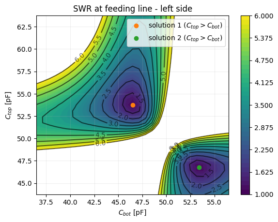
In order to illustrate the convergence, we first calculate a capacitor map \(\mathrm{VSWR}(C_{top}, C_{bot})\) for the left side around the ideal match point:
[13]:
delta_Cs = np.linspace(-10, +10, num=31, endpoint=True)
[14]:
C_top_lefts, C_bot_lefts = np.meshgrid(C_match_sol1[0] + delta_Cs,
                                       C_match_sol1[1] + delta_Cs)
print(C_top_lefts.size)
961
[15]:
power = [1, 1e-12]  # small value on right side to avoid division by zero
phase = [0, 0]

vswrs = []
for (C_top, C_bot) in tqdm(np.nditer([C_top_lefts, C_bot_lefts]), total=C_top_lefts.size):
    _vswr = antenna.vswr_act(power, phase, Cs=[C_top, C_bot, 120, 120])
    vswrs.append(_vswr)
vswrs = np.array(vswrs).squeeze()
vswrs_left = vswrs[:,0].reshape(C_top_lefts.shape)
Which looks like that:
[16]:
fig, ax = plt.subplots()
cs=ax.contourf(C_bot_lefts, C_top_lefts, vswrs_left, np.linspace(1, 6, 41))
cs2=ax.contour(C_bot_lefts, C_top_lefts, vswrs_left, np.linspace(1, 6, 11), colors='k', alpha=0.6)
ax.clabel(cs2, inline=1, fontsize=10)
ax.set_xlabel('$C_{bot}$ [pF]')
ax.set_ylabel('$C_{top}$ [pF]')
ax.set_title('SWR at feeding line - left side')
ax.grid(True, alpha=0.2)
ax.plot(C_match_sol1[1], C_match_sol1[0], 'o', color='C1', label="solution 1 ($C_{top} > C_{bot}$)")
ax.plot(C_match_sol2[1], C_match_sol2[0], 'o', color='C2', label="solution 2 ($C_{top} > C_{bot}$)")
ax.legend()
fig.colorbar(cs)
[16]:
<matplotlib.colorbar.Colorbar at 0x73da6b464b30>
Now let’s define a starting point and iterate on the capacitor predictor. Playing with the code below, you’ll see rapidly that the convergence is heavily linked to the starting point. Using a starting point far from the expected solution or with capacitor inversed with respected to the desired solution will lead to the divergence of the algorithm:
[17]:
C0_start = [60,40,120,120]
sol_num = 1

C0 = list(C0_start)  # new list to avoid reference
C0s = []
cont = True
iterations = 0
while cont:
    C_next_left, C_next_right, eps = antenna.capacitor_predictor(power, phase, Cs=C0, solution_number=sol_num)
    C0 = [C_next_left.squeeze()[0], C_next_left.squeeze()[1], 120, 120]

    iterations += 1
    if iterations > 1 and (np.abs(C0s[-1][0] - C0[0]) < 0.01) and (np.abs(C0s[-1][1] - C0[1]) < 0.01):
        cont = False
    if iterations > 60:
        cont = False
    C0s.append([C0[0], C0[1]])
print(f'Stopped after {iterations} iterations')
Stopped after 21 iterations
Let’s illustrate the trace of the matching convergence:
[18]:
fig, ax = plt.subplots()
cs=ax.contourf(C_bot_lefts, C_top_lefts, vswrs_left, np.linspace(1, 6, 41))
cs2=ax.contour(C_bot_lefts, C_top_lefts, vswrs_left, np.linspace(1, 6, 11), colors='k', alpha=0.6)
ax.clabel(cs2, inline=1, fontsize=10)
ax.set_xlabel('$C_{bot}$ [pF]')
ax.set_ylabel('$C_{top}$ [pF]')
ax.set_title('SWR at feeding line - left side')
ax.grid(True, alpha=0.2)
ax.plot(C_match_sol1[1], C_match_sol1[0], 'o', color='C1', label="solution 1 ($C_{top} > C_{bot}$)")
ax.plot(C_match_sol2[1], C_match_sol2[0], 'o', color='C2', label="solution 2 ($C_{top} > C_{bot}$)")
ax.legend()
fig.colorbar(cs)


C0s = np.array(C0s)
ax.plot(C0_start[1], C0_start[0], 'x', color='r')
ax.plot(C0s[:,1], C0s[:,0], '-x', color='r', alpha=0.8)
print(C0s[-1])
[53.61809454 46.55309157]

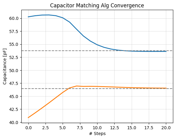
Below is another representation of the convergence:
[19]:
fig, ax = plt.subplots()
ax.plot(np.arange(len(C0s)), C0s, lw=2)
ax.set_xlabel('# Steps')
ax.set_ylabel('Capacitance [pF]')
ax.grid(True, alpha=.4)
ax.set_title('Capacitor Matching Alg Convergence')
ax.axhline(eval(f'C_match_sol{sol_num}')[0], ls='--', color='gray')
ax.axhline(eval(f'C_match_sol{sol_num}')[1], ls='--', color='gray')
[19]:
<matplotlib.lines.Line2D at 0x73da6e598590>
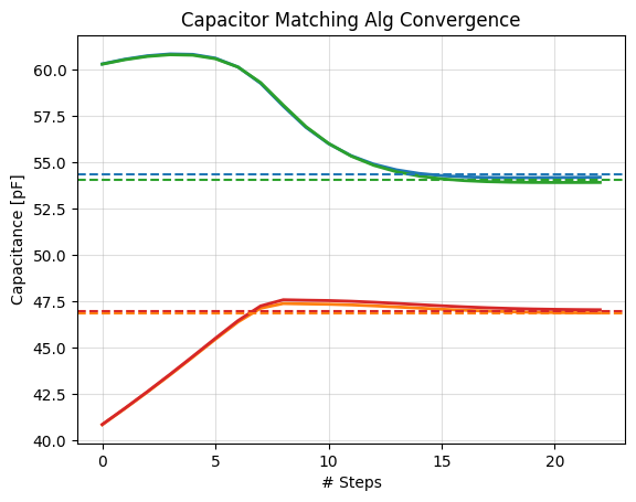
Matching both sides at the same time
[20]:
power = [1, 1]
phase = [0, np.pi]
# reference solution we wish to obtain
C_opt_dipole = antenna.match_both_sides(f_match=55e6, power=power, phase=phase)
Looking for individual solutions separately for 1st guess...
Wrong solution found ! Re-doing...
False solution #1: [150. 150.]
Wrong solution found ! Re-doing...
False solution #1: [150. 150.]
Wrong solution found ! Re-doing...
False solution #1: [150. 150.]
Wrong solution found ! Re-doing...
False solution #1: [150. 150.]
Wrong solution found ! Re-doing...
False solution #1: [150. 150.]
True solution #1: [53.75338416 46.49027248]
True solution #1: [53.37708094 46.64643417]
Searching for the active match point solution...
Reducing search range to +/- 5pF around individual solutions
True solution #1: [54.35732273 46.82037048 54.07852663 46.98665993]
[21]:
C0_start = [60, 40, 60, 40] # note that the start point matches solution 1 (Ctop>Cbot)
sol_num = 1

C0 = list(C0_start)  # new list to avoid reference
C0s = []
cont = True
iterations = 0
while cont:
    C_next_left, C_next_right, eps = antenna.capacitor_predictor(power, phase, Cs=C0, solution_number=sol_num)
    C0 = [C_next_left.squeeze()[0], C_next_left.squeeze()[1],
          C_next_right.squeeze()[0], C_next_right.squeeze()[1]]
    print(C0)
    iterations += 1
    if iterations > 1 and (np.abs(C0s[-1][0] - C0[0]) < 0.01) and (np.abs(C0s[-1][1] - C0[1]) < 0.01):
        cont = False
    if iterations > 60:
        cont = False
    C0s.append([C0[0], C0[1], C0[2], C0[3]])
print(f'Stopped after {iterations} iterations')
[np.float64(60.309880353554675), np.float64(40.8350147996163), np.float64(60.29662669754911), np.float64(40.845843731749305)]
[np.float64(60.564273172320405), np.float64(41.7003362343722), np.float64(60.539606904192794), np.float64(41.72087070647744)]
[np.float64(60.75035795609627), np.float64(42.596263351328204), np.float64(60.71656501163106), np.float64(42.62546121626117)]
[np.float64(60.847986873840135), np.float64(43.52262189086172), np.float64(60.80835065578185), np.float64(43.55957821913247)]
[np.float64(60.824197706203314), np.float64(44.47651174740701), np.float64(60.784100581472025), np.float64(44.52083218203285)]
[np.float64(60.6226014198148), np.float64(45.444962812302236), np.float64(60.591721554706275), np.float64(45.49831676960863)]
[np.float64(60.145933362705755), np.float64(46.37976539396375), np.float64(60.14149206389021), np.float64(46.45168615186622)]
[np.float64(59.26241007831531), np.float64(47.12105459295298), np.float64(59.30334428978761), np.float64(47.24409063820389)]
[np.float64(58.03052021258051), np.float64(47.37606630841939), np.float64(58.09002644687563), np.float64(47.57768041359946)]
[np.float64(56.887217288304385), np.float64(47.35421960005617), np.float64(56.93120824024291), np.float64(47.553381675442644)]
[np.float64(56.00704069980338), np.float64(47.33793066976474), np.float64(56.02234200815716), np.float64(47.53489897201158)]
[np.float64(55.35637813617794), np.float64(47.30256488841006), np.float64(55.334677161107365), np.float64(47.497750235089)]
[np.float64(54.899258471588915), np.float64(47.25200754912421), np.float64(54.836603343144816), np.float64(47.445093567741175)]
[np.float64(54.59321530014588), np.float64(47.191551196040265), np.float64(54.48968115338548), np.float64(47.38230799820948)]
[np.float64(54.397955577995376), np.float64(47.127775841648244), np.float64(54.256594028877814), np.float64(47.31599177864086)]
[np.float64(54.280018570258655), np.float64(47.06662555610448), np.float64(54.10560871597316), np.float64(47.25212016184422)]
[np.float64(54.213927513302465), np.float64(47.0123008203427), np.float64(54.01188158058262), np.float64(47.19496312262823)]
[np.float64(54.18130926402249), np.float64(46.96704171186901), np.float64(53.95691265030345), np.float64(47.14687436894319)]
[np.float64(54.169359506379735), np.float64(46.93144461016859), np.float64(53.92734949683574), np.float64(47.108585286741956)]
[np.float64(54.16937937264233), np.float64(46.904960389292285), np.float64(53.91377517745098), np.float64(47.07967007735798)]
[np.float64(54.17561340614429), np.float64(46.88637223524739), np.float64(53.90969846837462), np.float64(47.05899875267516)]
[np.float64(54.1843891826048), np.float64(46.8741743289644), np.float64(53.91077139980983), np.float64(47.04510591066693)]
[np.float64(54.19349220363589), np.float64(46.86683780157356), np.float64(53.91419640731545), np.float64(47.03645962826116)]
Stopped after 23 iterations
[22]:
fig, ax = plt.subplots()
ax.plot(np.arange(len(C0s)), C0s, lw=2)
ax.set_xlabel('# Steps')
ax.set_ylabel('Capacitance [pF]')
ax.grid(True, alpha=.4)
ax.set_title('Capacitor Matching Alg Convergence')
[ax.axhline(C, ls='--', color=f'C{idx}') for idx, C in enumerate(C_opt_dipole)]
[22]:
[<matplotlib.lines.Line2D at 0x73da6e5984a0>,
 <matplotlib.lines.Line2D at 0x73da691c7a10>,
 <matplotlib.lines.Line2D at 0x73da6e7463f0>,
 <matplotlib.lines.Line2D at 0x73da693e0fb0>]
The antenna is matched:
[23]:
antenna.vswr_act(power, phase, Cs=C0s[-1])
[23]:
array([1.05743152, 1.05556392])
The automatic matching algorithm is implemented in the matching_both_sides_iterative method of the antenna object:
[24]:
C_opt_2 = antenna.match_both_sides_iterative(f_match=55e6, power=power, phase=phase, Cs=[50, 50, 50, 50])
Stopped after 15 iterations
Solution found: [np.float64(54.24420285827658), np.float64(46.86180303696939), np.float64(53.94828608941629), np.float64(47.02701519647144)]
[25]:
antenna.vswr_act(power, phase, Cs=C_opt_2)
[25]:
array([1.04158968, 1.04131346])
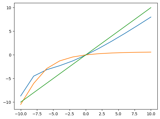
Correspondance Between Error Signal Amplitude and Capacitance
In the control room, the IC operator job is often to improve the antenna tuning for the next shot. Because turning on the matching feedback is not always desirable, another option is to look to the error signals \(\mathbf{\varepsilon}\) generated in the latest pulse and to deduce from them the correction to apply to the capacitors.
First, let’s build a half-matched antenna:
[26]:
f0 = 55  # MHz
freq0 = rf.Frequency(f0, f0, unit='MHz', npoints=1)
antenna = WestIcrhAntenna(frequency=freq0,
                          front_face='../west_ic_antenna/data/Sparameters/front_faces/TOPICA/S_TSproto12_55MHz_Hmode_LAD6-2.5cm.s4p')
C_match = antenna.match_one_side(f_match=f0*1e6,
                                 side='left', solution_number=1)
print(C_match)
Wrong solution found ! Re-doing...
False solution #1: [150. 150.]
True solution #1: [53.75337803 46.49027141]
[np.float64(53.753378033599134), np.float64(46.49027140849695), 150, 150]
Now, let’s depart one capacitor from the ideal point and look to the evolution of the error signal:
[27]:
delta_Cs = np.linspace(-10, +10, 11)

_Cs = []
for delta_C in tqdm(delta_Cs):
    Cs = [C_match[0]+delta_C, *C_match[1:]]
    _C = antenna.capacitor_predictor(power, phase, Cs)[0].squeeze()
    _Cs.append(_C)
_Cs = np.array(_Cs)
[28]:
fig, ax = plt.subplots()
ax.plot(delta_Cs, _Cs-C_match[:2])
ax.plot([-10, 10], [-10, 10])
[28]:
[<matplotlib.lines.Line2D at 0x73da6e5a9ac0>]
Velocity Controler
The velocity controler matrix \(\mathbf{T}\) is in fact \(\mathbf{D}^{-1}\), since the velocity \(\mathbf{V}\) is proportional to the change \(\delta C\):
so that
Following the previous result on \(\mathbf{D}\), the matrix \(\mathbf{T}\) can be parametrized as:
Where \(k\) is gain, \(S\) and \(\alpha\) two parameters used to define the choice of the matching solution (“1” for \(C_{top}>C_{bot}\), “2” for the opposite). \(K_{ri}\) is used to define the relative weight between real and imaginary part of the error signal \(\mathbf{\varepsilon}\).
[29]:
from IPython.core.display import HTML
def _set_css_style(css_file_path):
    """
    Read the custom CSS file and load it into Jupyter
    Pass the file path to the CSS file
    """
    styles = open(css_file_path, "r").read()
    s = '<style>%s</style>' % styles
    return HTML(s)

_set_css_style('custom.css')
[29]:
[ ]: