Phase Scan Effect on Antenna Voltage Unbalance

In this notebook we explore the effect of a phase scan over the voltage unbalance.

%load_ext autoreload
%autoreload 2

import matplotlib.pyplot as plt
import numpy as np
import skrf as rf
from tqdm.notebook import tqdm

# WEST ICRH Antenna package
import sys; sys.path.append('..')
from west_ic_antenna import WestIcrhAntenna

# nicer plot
rf.stylely()

Let’s use a TOPICA simulation of the WEST front face in a “L-mode plasma” at 55 MHz:

freq = rf.Frequency(start=50, stop=60, npoints=1001, unit='MHz')
plasma_TOPICA = '../west_ic_antenna/data/Sparameters/front_faces/TOPICA/S_TSproto12_55MHz_Hmode_LAD6-2.5cm.s4p'

antenna = WestIcrhAntenna(frequency=freq, front_face=plasma_TOPICA)
print(f'Optimal coupling resistance expected:', antenna.front_face_Rc().max())

Optimal coupling resistance expected: 1.6095500081638652

First, we match the antenna, both sides at the same time to operate the antenna at 55 MHz.

# antenna excitation to match for
power = [1, 1]  # W
phase = [0, np.pi]  # dipole

Cs = antenna.match_both_sides(f_match=55e6, power=power, phase=phase,
                              solution_number=1, verbose=False)

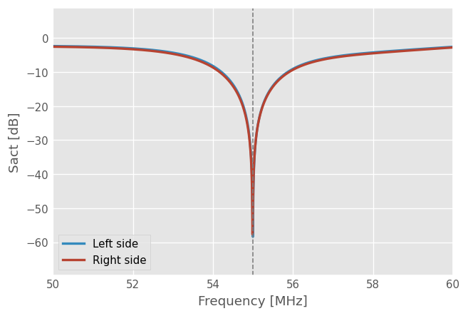
Let’s visualize how good the antenna is matched for the target frequency, by looking to the active S parameters (ie. taking into account the antenna excitation)

s_act = antenna.s_act(power=power, phase=phase, Cs=Cs)

fig, ax = plt.subplots()
ax.plot(antenna.f_scaled, 20*np.log10(np.abs(s_act)), lw=2)
ax.set_xlabel('Frequency [MHz]')
ax.set_ylabel('Sact [dB]')
ax.legend(('Left side', 'Right side'))
ax.axvline(55, ls='--', color='gray')

<matplotlib.lines.Line2D at 0x7ddfe8b394f0>

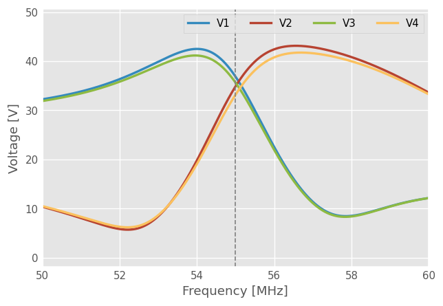
Now that the antenna is perfeclty matched, let’s see how the voltages evolve with frequency. At the match frequency, the voltages (and currents) get very close: the antenna is balanced.

fig, ax = plt.subplots()
ax.plot(antenna.f_scaled, np.abs(antenna.voltages(power, phase, Cs)), lw=2)
ax.axvline(55, ls='--', color='gray')
ax.set_xlabel('Frequency [MHz]')
ax.set_ylabel('Voltage [V]')
ax.legend(('V1', 'V2', 'V3', 'V4'), ncol=4)

<matplotlib.legend.Legend at 0x7ddfe5fbd190>

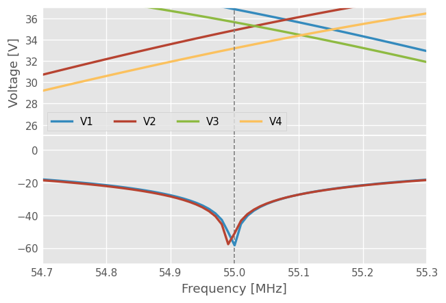
Note that the antenna voltages are not perfectly balanced at the match point, which is expected due to the intercouplings:

fig, (ax1,ax2) = plt.subplots(2, 1, sharex=True)
ax1.plot(antenna.f_scaled, np.abs(antenna.voltages(power, phase, Cs)), lw=2)
[a.axvline(55, ls='--', color='gray') for a in (ax1,ax2)]
ax2.set_xlabel('Frequency [MHz]')
ax1.set_ylabel('Voltage [V]')
ax1.legend(('V1', 'V2', 'V3', 'V4'), ncol=4)
ax1.set_xlim(54.7, 55.3)
ax1.set_ylim(25, 37)
ax2.plot(antenna.f_scaled, 20*np.log10(np.abs(s_act)), lw=2)
fig.subplots_adjust(hspace=0)

So let’s see how the voltages evolve at the match frequency when we sweep the phase shift between sides:

power = [1e6, 1e6]  # 1 MW each side
toroidal_phases = np.deg2rad(np.linspace(start=0, stop=360, num=36))

antenna_single_freq = WestIcrhAntenna(frequency=rf.Frequency(55, 55, 1, unit='MHz'),
                                     front_face=plasma_TOPICA, Cs=Cs)

voltages, currents, Rcs = [], [], []
for toroidal_phase in tqdm(toroidal_phases):
    voltages.append(antenna_single_freq.voltages(power, phase=[0, toroidal_phase]))
    currents.append(antenna_single_freq.voltages(power, phase=[0, toroidal_phase]))
    Rcs.append(antenna_single_freq.Rc_WEST(power, phase=[0, toroidal_phase]))
voltages = np.array(voltages).squeeze()
currents = np.array(currents).squeeze()
Rcs = np.array(Rcs).squeeze()

# export data
np.savetxt('voltages_vs_phase.csv',
           np.c_[np.rad2deg(toroidal_phases), np.abs(voltages)])

fig, ax = plt.subplots()
ax.plot(np.rad2deg(toroidal_phases), np.abs(voltages)/1e3, lw=2)
ax.axvline(180, ls='--', color='gray')
ax.set_xlabel('Toroidal Phase [deg]')
ax.set_ylabel('Voltage [kV]')
ax.legend(('V1', 'V2', 'V3', 'V4'), ncol=4)
ax.set_ylim(0,50)

(0.0, 50.0)

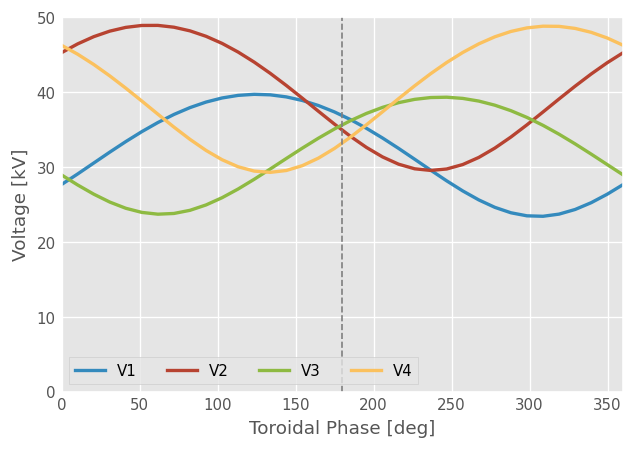
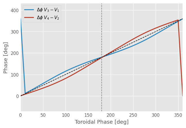
The phase sweep generates voltage (or currents) unbalance.

The voltage probe toroidal phase difference is also slightly affected in this case:

fig, ax = plt.subplots()
ax.plot(np.rad2deg(toroidal_phases), np.rad2deg(np.angle(voltages[:,2]) - np.angle(voltages[:,0]))%360, lw=2)
ax.plot(np.rad2deg(toroidal_phases), np.rad2deg(np.angle(voltages[:,3]) - np.angle(voltages[:,1]))%360, lw=2)
ax.plot(np.rad2deg(toroidal_phases), np.rad2deg(toroidal_phases), color='k', ls='--')
ax.axvline(180, ls='--', color='gray')
ax.set_xlabel('Toroidal Phase [deg]')
ax.set_ylabel('Phase [deg]')
ax.legend(('$\Delta  \phi$ $V_3-V_1$', '$\Delta  \phi$ $V_4-V_2$'))

<>:8: SyntaxWarning: invalid escape sequence '\D'
<>:8: SyntaxWarning: invalid escape sequence '\D'
<>:8: SyntaxWarning: invalid escape sequence '\D'
<>:8: SyntaxWarning: invalid escape sequence '\D'
/tmp/ipykernel_2664/267035272.py:8: SyntaxWarning: invalid escape sequence '\D'
  ax.legend(('$\Delta  \phi$ $V_3-V_1$', '$\Delta  \phi$ $V_4-V_2$'))
/tmp/ipykernel_2664/267035272.py:8: SyntaxWarning: invalid escape sequence '\D'
  ax.legend(('$\Delta  \phi$ $V_3-V_1$', '$\Delta  \phi$ $V_4-V_2$'))

<matplotlib.legend.Legend at 0x7ddfe63c0a10>

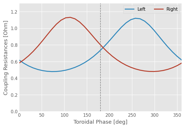
Coupling resistance, which is deduced from the currents, is of course also affected:

fig, ax = plt.subplots()
ax.plot(np.rad2deg(toroidal_phases), Rcs, lw=2)
ax.axvline(180, ls='--', color='gray')
ax.set_xlabel('Toroidal Phase [deg]')
ax.set_ylabel('Coupling Resistances [Ohm]')
ax.legend(('Left', 'Right'), ncol=4)
ax.set_ylim(0,1.3)

(0.0, 1.3)

from IPython.core.display import HTML
def _set_css_style(css_file_path):
    """
    Read the custom CSS file and load it into Jupyter
    Pass the file path to the CSS file
    """
    styles = open(css_file_path, "r").read()
    s = '<style>%s</style>' % styles
    return HTML(s)

_set_css_style('custom.css')