Introduction

The WEST ICRH antennas

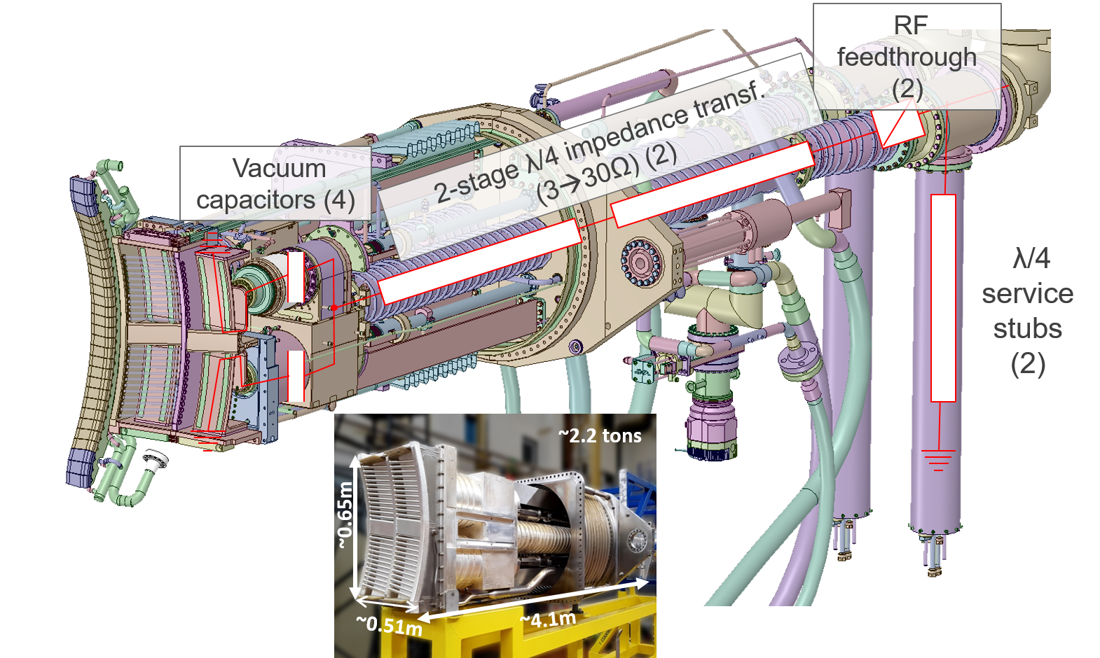
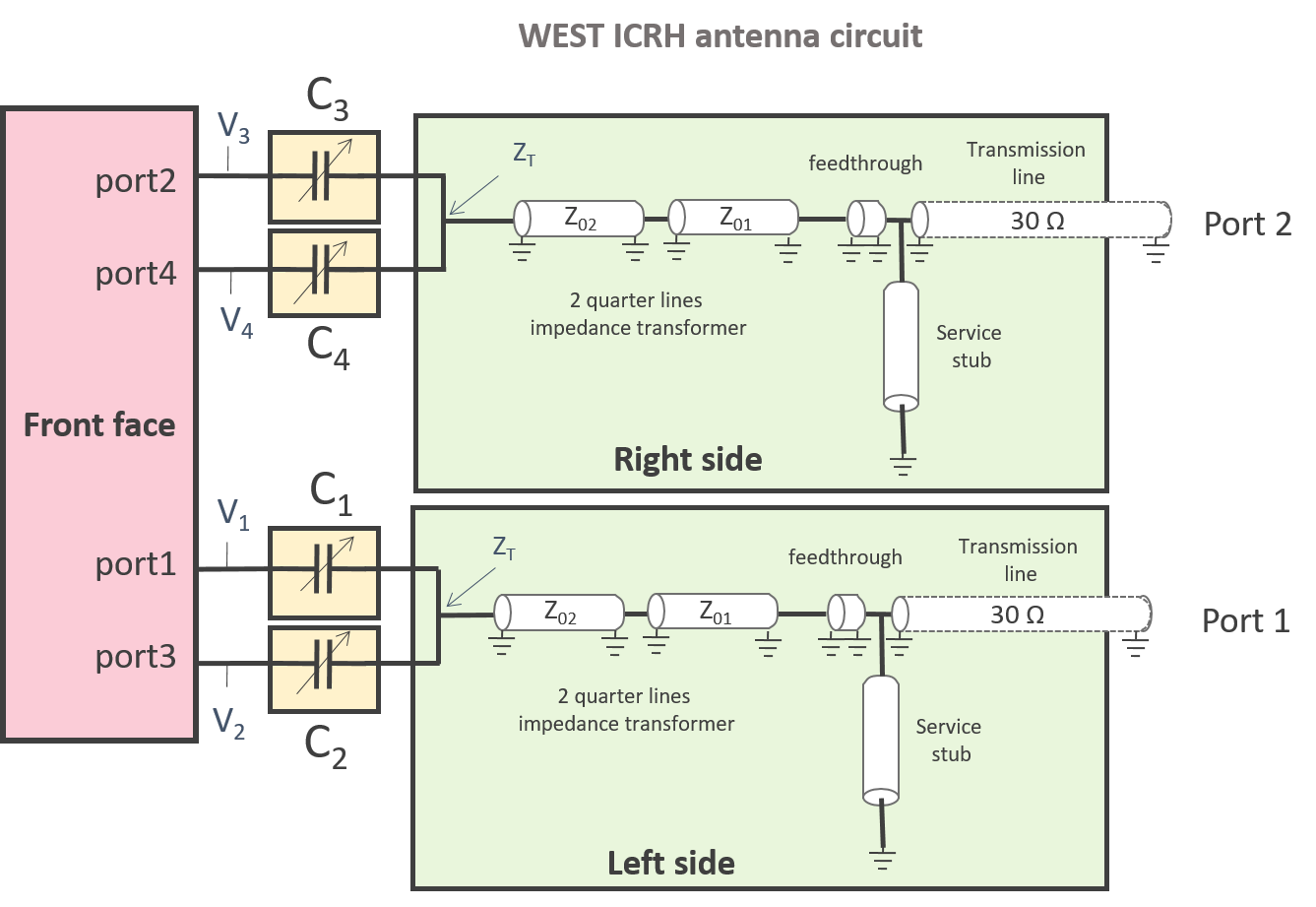
Three identical ELM-resilient and CW power ICRH antennas have been designed for WEST. The ELM resilience property is obtained through an internal conjugate-T electrical scheme with series capacitors. An antenna has 4 straps (2 toroidal x 2 poloidal) and is fed by 2 generators (left side and right side). Each antenna is equipped with four internal COMET® tuneable vacuum capacitors, with capacitances ranging from 15 pF to 150 pF and specifically upgraded for CW operation. A two-stage quarter-wavelength and water cooled impedance transformer is connected from the T-junction to the vacuum feedthrough.

WEST IC antenna Python RF Model

%load_ext autoreload
%autoreload 2

import matplotlib.pyplot as plt
import numpy as np
import skrf as rf
rf.stylely()  # pretty plots
from tqdm.notebook import tqdm
# WEST ICRH Antenna package
import sys; sys.path.append('..')
from west_ic_antenna import WestIcrhAntenna

The WEST ICRH Antenna RF model can be built by defining one or all of:

• the frequency band of interest, given by a scikit-rf Frequency object

• the front face (Touchstone) S-parameter filename, ie. the model of the antenna front-face radiating to a given medium (or a scikit-rf 4-port Network)

• the capacitor’s capacitances [C1, C2, C3, C4]

All these parameters are optionnal when builing the WestIcrhAntenna object. Default parameters is a frequency band 30-70 MHz, with the front-face radiating in vacuum with all capacitances set to 50 pF.

# Using default values
antenna = WestIcrhAntenna()
print(antenna)

WEST ICRH Antenna: C=[50, 50, 50, 50] pF, 0.03-0.07 GHz, 4001 pts

For example, to reduce the frequency band of interest:

freq = rf.Frequency(48, 57, npoints=2001, unit='MHz')
antenna = WestIcrhAntenna(frequency=freq)

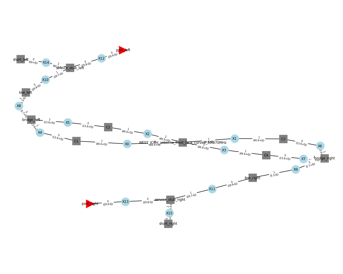
The antenna circuit can be visualized via the scikit-rf Circuit object:

antenna.circuit().plot_graph(network_labels=True, edge_labels=True,
inter_labels=True, port_labels=True)

Antenna Matching

Matching the WEST ICRH antenna consists in setting up the 4 capacitances values (\(C_1,C_2,C_3,C_4\)) to achieve the desired behaviour, typically a low reflected power to the generators. For the given geometry of the WEST antenna, these optimal capacitances depend on:

• the antenna front-face, i.e. the plasma properties facing the antenna;

• the antenna excitation, powers and phasing between left and right sides.

Matching the antenna in one step

The optimum set of capacitances to minimize the reflected power at a given frequency can be obtained using the match_both_sides() method:

f_match = 55e6
C_match = antenna.match_both_sides(f_match=f_match)

Looking for individual solutions separately for 1st guess...
Wrong solution found ! Re-doing...
False solution #1: [150. 150.]
Wrong solution found ! Re-doing...
False solution #1: [150. 150.]
True solution #1: [51.44282966 49.32526853]
Wrong solution found ! Re-doing...
False solution #1: [38.00686072 12.        ]
True solution #1: [51.20961665 49.48963479]
Searching for the active match point solution...
Reducing search range to +/- 5pF around individual solutions
True solution #1: [52.09601242 50.08043849 51.62213165 50.2573231 ]

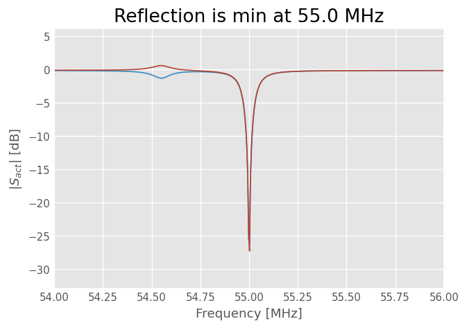
# dipole excitation for the set of capacitances
power = [1, 1]
phase = [0, np.pi]

# Antenna reflection coefficient in dB (active S-parameter, cf next section)
s_act_db = antenna.s_act_db(power, phase, C_match)

fig, ax = plt.subplots()
ax.plot(antenna.f_scaled, s_act_db)
ax.set_xlabel('Frequency [MHz]')
ax.set_ylabel('$|S_{act}|$ [dB]')
ax.set_title(f'Reflection is min at {f_match/1e6} MHz')
ax.set_xlim(54, 56)

/home/docs/checkouts/readthedocs.org/user_builds/west-ic-antenna/checkouts/latest/doc/../west_ic_antenna/antenna.py:1316: FutureWarning: skrf.mag_2_db is deprecated. Please import mag_2_db from skrf.mathFunctions instead.
  return rf.mag_2_db(np.abs(self.s_act(power, phase, Cs)))

(54.0, 56.0)

Matching the antenna step by step

When both sides of the antenna are used (which is the desired situation), the figure of merit is not the reflection coefficient from scattering parameters (such as \(S_{11}\) or \(S_{22}\)) but the “active” parameters, that is the RF parameters taking into account the antenna feeding and cross-coupling effects between both sides. Because of these cross-coupling effects, the matching point for each side used separately is not the same than for both sides used together.

Let’s see step by step these effects.

Each side of the antenna can be matched separately, which is what is done in practice since it’s simpler to act on two capacitors than four at the same time.

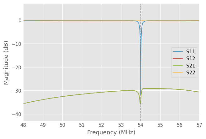
Let’s start with the left side, looking for a solution at 54 MHz, with the solution 1 (corresponding to \(C_{top} > C_{bot}\), solution 2 being the opposite). The right side is left unmatched.

f_match = 54e6
C_match_left = antenna.match_one_side(f_match=f_match,
                                      side='left', solution_number=1)

Wrong solution found ! Re-doing...
False solution #1: [150. 150.]
True solution #1: [54.50609392 52.20484949]

Once the solution has been found, we setup the antenna capacitors to these values:

antenna.Cs = C_match_left

Let’s have a look to the S-parameters of the antenna, which is a 2-port network. An easy way to plot them is to retrieve the scikit-rf Network object and its convenience methods:

fig, ax = plt.subplots()
antenna.circuit().network.plot_s_db(ax=ax)
ax.axvline(f_match, color='gray', ls='--')

<matplotlib.lines.Line2D at 0x71cd27a6c590>

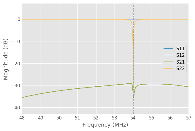
Now let’s match the right side (the left side being unmatched). This time, it will minimize the S22 at the match frequency.

C_match_right = antenna.match_one_side(f_match=f_match,
                                       side='right', solution_number=1)
antenna.Cs = C_match_right
fig, ax = plt.subplots()
antenna.circuit().network.plot_s_db(ax=ax)
ax.axvline(f_match, color='gray', ls='--')

Wrong solution found ! Re-doing...
False solution #1: [150. 150.]
Wrong solution found ! Re-doing...
False solution #1: [150. 150.]
Wrong solution found ! Re-doing...
False solution #1: [150. 150.]
True solution #1: [54.26438301 52.37610949]

<matplotlib.lines.Line2D at 0x71cd27ab4230>

If we setup the antenna with the combination of these two solutions, and zoom into the 48-52 MHz band, one sees that antenna shows two optimized frequencies around the match frequencies.

C_match = [C_match_left[0], C_match_left[1], C_match_right[2], C_match_right[3]]
print(C_match)
antenna.Cs = C_match

[np.float64(54.50609391935816), np.float64(52.204849486064646), np.float64(54.26438300768323), np.float64(52.3761094872545)]

fig, ax = plt.subplots()
antenna.circuit(Cs=C_match).network.plot_s_db(ax=ax)
ax.axvline(f_match, color='gray', ls='--')

<matplotlib.lines.Line2D at 0x71cd2b364230>

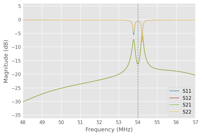
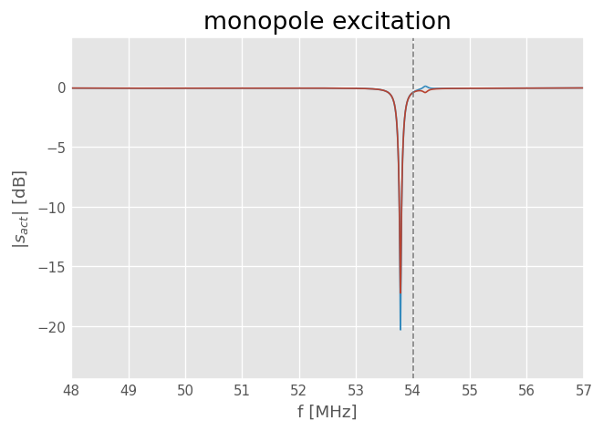
These optimum frequencies correspond to the monopole and dipole excitations. Instead of looking to the S-parameters, it is more meaningfull to look to the active S-parameters, defined by:

\[S_{act,m} = \sum_{n=1}^M S_{mn} \frac{a_n}{a_m}\]

with \(m=1..N\) where \(N\) is the number of ports (here M=2) and \(a_k\) the complex excitation for the k-th port.

# monopole excitation, left side being the reference
power = [1, 1]
phase = [0, 0]
# getting the active s-parameters
s_act_db = antenna.s_act_db(power, phase)
# plotting
fig, ax = plt.subplots()
ax.plot(freq.f_scaled, s_act_db)
ax.axvline(f_match/1e6, ls='--', color='gray')
ax.set_title('monopole excitation')
ax.set_xlabel('f [MHz]')
ax.set_ylabel('$|s_{act}|$ [dB]')
ax.grid(True)

/home/docs/checkouts/readthedocs.org/user_builds/west-ic-antenna/checkouts/latest/doc/../west_ic_antenna/antenna.py:1316: FutureWarning: skrf.mag_2_db is deprecated. Please import mag_2_db from skrf.mathFunctions instead.
  return rf.mag_2_db(np.abs(self.s_act(power, phase, Cs)))

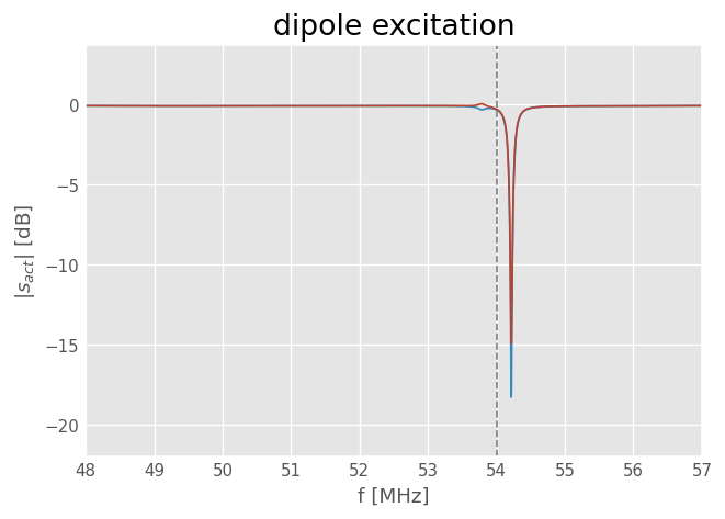
# dipole excitation, left side being the reference
power = [1, 1]
phase = [0, np.pi]
# getting the active s-parameters
s_act_db = antenna.s_act_db(power, phase, Cs=C_match)
# plotting
fig, ax = plt.subplots()
ax.plot(freq.f_scaled, s_act_db)
ax.axvline(f_match/1e6, ls='--', color='gray')
ax.set_title('dipole excitation')
ax.set_xlabel('f [MHz]')
ax.set_ylabel('$|s_{act}|$ [dB]')
ax.grid(True)

Voltages and Currents

# dipole case, 1 MW input on both sides
power = [1e6, 1e6]
phase = [0, np.pi]

Vs = antenna.voltages(power, phase)
Is = antenna.currents(power, phase)

fig, ax = plt.subplots(2,1,sharex=True)
ax[0].plot(freq.f_scaled, np.abs(Vs)/1e3)
ax[1].plot(freq.f_scaled, np.abs(Is)/1e3)
ax[1].set_xlabel('f [MHz]')
ax[0].set_ylabel('Voltage [kV]')
ax[1].set_ylabel('Current [kA]')
[a.grid(True) for a in ax]
ax[0].legend(('V1','V2','V3','V4'))
ax[1].legend(('I1','I2','I3','I4'))

<matplotlib.legend.Legend at 0x71cd2b6e14f0>

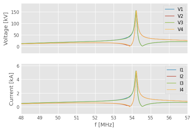
The voltage and current values are of course not realistic, because the antenna is radiating on vacuum here, not on plasma.

Impedance at the T-junction

The WEST ICRH antennas design is based on the conjugate-T to insure a load-tolerance. In particular, they have been designed to operate with an impedance at the T-junction \(Z_T\) close to 3 Ohm. An impedance transformer connects the T-junction to the feeding transmission line (30 Ohm line). Hence, matching the antenna is similar to having a 30 Ohm load connected to the feeding transmission line, such as no power is reflected (VSWR\(\to 1\)), which should be equivalent of having an impedance of roughtly 3 Ohm at the T-junction.

However, due to real-life design and manufacturing constraints, the optimal impedance at the T-junction is not necessarely 3 Ohm, but can be slightly different in both real and imaginary parts.

So let’s evaluate the impact of the realistic geometries (simulated from full-wave tools) on the impedance at the T-junction to the 30 Ohm feeder line (the one which really matter for the generator point-of-view).

For that, let’s take the impedance transformer/vacuum window/service stub network assembly of an antenna:

freq = rf.Frequency(50, 50, unit='MHz', npoints=1)
antenna = WestIcrhAntenna(frequency=freq)
assembly = antenna.windows_impedance_transformer
# note that port 1 corresponds to the generator side (30 Ohm)
print(assembly)

2-Port Network: 'WEST_ICRH_Transf_Window_PumpHolePMC',  50.0-50.0 MHz, 1 pts, z0=[29.89491473-0.00316299j  5.2989722 -0.00376783j]

The port 1 of this network assembly corresponds to the 30 Ohm feeding line while the port 2 correspond to the end of the second section of the impedance transformer. Let’s load the port 2 with an ideal impedance \(Z_T=R_T + j X_T\) and scanning the effect of \(R_T\) and \(X_T\) on the VSWR seen by the generator.

# create a grid of R_T and X_T values
R_Ts, X_Ts = np.meshgrid(np.linspace(1, 5, 50),
                         np.linspace(-3, 3, 50))
media_port2 = rf.DefinedGammaZ0(frequency=freq, z0=assembly.z0[:,1].real)

/home/docs/checkouts/readthedocs.org/user_builds/west-ic-antenna/checkouts/latest/.venv/lib/python3.12/site-packages/skrf/__init__.py:75: FutureWarning: skrf.io.DefinedGammaZ0 is deprecated. Please import DefinedGammaZ0 from skrf.io.touchstone instead.
  result = getattr(module, name, None)
/tmp/ipykernel_2444/2902204356.py:4: FutureWarning: skrf.DefinedGammaZ0 is deprecated. Please import DefinedGammaZ0 from skrf.io instead.
  media_port2 = rf.DefinedGammaZ0(frequency=freq, z0=assembly.z0[:,1].real)

# calculate the VSWR at port 1 as a function of (R_T, X_T)
vswrs = []
for (R_T,X_T) in tqdm(np.nditer([R_Ts, X_Ts])):
    Z_T = R_T + 1j*X_T
    # connect the port 2 with a impedance Z_T
    ntw = assembly ** media_port2.load(rf.zl_2_Gamma0(assembly.z0[:,1].real, Z_T))
    vswrs.append(ntw.s_vswr)
# reshape to 2D
vswrs = np.array(vswrs).reshape(R_Ts.shape)

/tmp/ipykernel_2444/2790215702.py:6: FutureWarning: skrf.zl_2_Gamma0 is deprecated. Please import zl_2_Gamma0 from skrf.tlineFunctions instead.
  ntw = assembly ** media_port2.load(rf.zl_2_Gamma0(assembly.z0[:,1].real, Z_T))
/home/docs/checkouts/readthedocs.org/user_builds/west-ic-antenna/checkouts/latest/.venv/lib/python3.12/site-packages/skrf/network.py:5758: UserWarning: Connecting two networks with different s_def and complex ports. The resulting network will have s_def of the first network: traveling. To silence this warning explicitly convert the networks to same s_def using `renormalize` function.
  return connect(ntwkA, N, ntwkB, 0)

fig, ax = plt.subplots()
cs=ax.contour(R_Ts, X_Ts, vswrs,
             np.linspace(1, 2, 21))
ax.clabel(cs, inline=1, fontsize=10)
ax.set_xlabel('R_T [Ohm]')
ax.set_ylabel('X_T [Ohm]')
ax.set_title('SWR at feeding line')
ax.axvline(3, color='gray', alpha=0.8)
ax.axhline(0, color='gray', alpha=0.8)
ax.grid(True, alpha=0.2)
ax.axis([0, 6, -2.2, 2.2])
ax.set_aspect('equal')

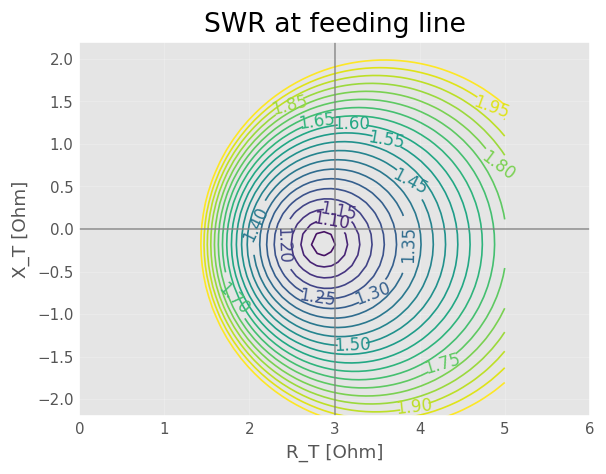
Hence the optimal impedance at the T-junction is not 3 Ohm, but slightly close in the complex plane. Let’s calculate this optimal value using:

from scipy.optimize import minimize

assembly.s_def = 'power'
def optim_fun(x):
    R_T, X_T = x
    Z_T = R_T + 1j*X_T
    # connect the port 2 with a impedance Z_T
    ntw = assembly ** media_port2.load(rf.zl_2_Gamma0(assembly.z0[:,1].real, Z_T))
    return ntw.s_vswr.flatten()[0]

sol = minimize(optim_fun, x0=[3,0])
print('Optimum Z_T=', sol.x[0] + 1j*sol.x[1])

/tmp/ipykernel_2444/2630263593.py:6: FutureWarning: skrf.zl_2_Gamma0 is deprecated. Please import zl_2_Gamma0 from skrf.tlineFunctions instead.
  ntw = assembly ** media_port2.load(rf.zl_2_Gamma0(assembly.z0[:,1].real, Z_T))

Optimum Z_T= (2.8656500342027074-0.17293477561516896j)

/tmp/ipykernel_2444/2630263593.py:6: FutureWarning: skrf.zl_2_Gamma0 is deprecated. Please import zl_2_Gamma0 from skrf.tlineFunctions instead.
  ntw = assembly ** media_port2.load(rf.zl_2_Gamma0(assembly.z0[:,1].real, Z_T))

The optimum T-impedance is such \(Z_T= 2.87 - 0.17j\).

from IPython.core.display import HTML
def _set_css_style(css_file_path):
    """
    Read the custom CSS file and load it into Jupyter
    Pass the file path to the CSS file
    """
    styles = open(css_file_path, "r").read()
    s = '<style>%s</style>' % styles
    return HTML(s)

_set_css_style('custom.css')