Coupling to Ideal Loads

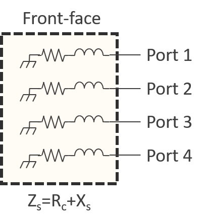
In this notebook, we investigate the WEST ICRH antenna behavior when the front-face is considered as the combination of ideal (and independent) loads made of impedances all equal to \(Z_s=R_c+j X_s\), where \(R_c\) corresponds to the coupling resistance and \(X_s\) is the strap reactance.

In such case, the power delivered to the plasma/front-face is then:

\[P_t = \frac{1}{2} \sum_{i=1}^4 \Re[V_i I_i^* ] = \frac{1}{2} \sum_{i=1}^4 \Re[Z_i] |I_i|^2 = \frac{1}{2} R_c \sum_{i=1}^4 |I_i|^2\]

Hence, we have defined the coupling resistance as:

\[R_c = \frac{\sum_{i=1}^4 \Re[Z_i] |I_i|^2}{\sum_{i=1}^4 |I_i|^2}\]

Inversely, the coupling resistance can be determined from:

\[R_c = \frac{2 P_t}{\sum_{i=1}^4 |I_i|^2}\]

In practice however, it is easier to measure RF voltages than currents.

\[I = \frac{V}{Z_s} = \frac{V}{R_c + j X_s} \rightarrow |I|^2 = \frac{|V|^2}{|R_c + j X_s|} \approx \frac{|V|^2}{|X_s|^2}\]

since in \(|X_s|>>|R_c|\).

The antenna model allows to calculate the coupling resistance from currents (.Rc() method) or from the voltage (.Rc_WEST() method).

The strap reactance \(X_s\) depends on the strap geometry and varies with the frequency. So, let’s find how the strap reactance from the realistic CAD model.

%matplotlib inline

import matplotlib.pyplot as plt
import numpy as np
import skrf as rf
from tqdm.notebook import tqdm

# WEST ICRH Antenna package
import sys; sys.path.append('..')
from west_ic_antenna import WestIcrhAntenna

# styling the figures
rf.stylely()

Coupling to an ideal front-face

Coupling to an ideal front face of coupling resistance \(R_c\) is easy using the the .load() method of the WestIcrhAntenna class. This method takes into account the strap reactance frequency fit (derived in Strap Reactance Frequency Fit)

freq = rf.Frequency(30, 70, npoints=1001, unit='MHz')
ant_ideal = WestIcrhAntenna(frequency=freq)
ant_ideal.load(Rc=1) # 1 Ohm coupling resistance front-face

# matching left and right sides : note that the solutions are (almost) the same
f_match = 55.5e6
C_left = ant_ideal.match_one_side(f_match=f_match, side='left')
C_right = ant_ideal.match_one_side(f_match=f_match, side='right')

Wrong solution found ! Re-doing...
False solution #1: [150. 150.]
True solution #1: [52.53812838 45.11248397]
Wrong solution found ! Re-doing...
False solution #1: [43.81834272 12.        ]
Wrong solution found ! Re-doing...
False solution #1: [150. 150.]
Wrong solution found ! Re-doing...
False solution #1: [150. 150.]
Wrong solution found ! Re-doing...
False solution #1: [150. 150.]
Wrong solution found ! Re-doing...
False solution #1: [150. 150.]
True solution #1: [52.53809903 45.11245951]

At the difference of the “real” situation (see the Matching or the Coupling to a TOPICA plasma), here is no poloidal neither toroidal coupling of the straps in this front-face model. This leads to:

• Match soluitions are the same for both sides (within \(10^{-3}\) pF).

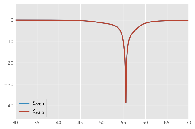
• Using the match solutions for each sides does not require to shift the operating frequency:

# dipole excitation
power = [1, 1]
phase = [0, np.pi]

# active S-parameter for the match point:
C_match = [C_left[0], C_left[1], C_right[2], C_right[3]]
s_act = ant_ideal.s_act(power, phase, Cs=C_match)

fig, ax = plt.subplots()
ax.plot(ant_ideal.f_scaled, 20*np.log10(np.abs(s_act)), lw=2)
ax.legend((r'$S_{act,1}$', r'$S_{act,2}$'))
ax.grid(True)

Match Points vs Coupling Resistance

Let’s determine the match points for a range of coupling resistance at a given frequency

f_match = 55e6
Rcs = np.r_[0.01, 0.05, np.arange(0.1, 2.0, 0.2)]

C_matchs = []
ant = WestIcrhAntenna()
for Rc in tqdm(Rcs):
    ant.load(Rc)
    C_match = ant.match_one_side(f_match=f_match, verbose=False, decimals=2)
    C_matchs.append(C_match)

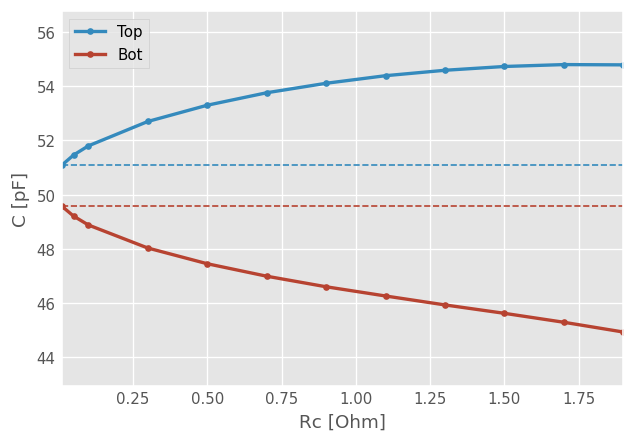
As the coupling resistance increases, the distance between capacitances (Top vs Bottom) increases:

fig, ax = plt.subplots()
ax.plot(Rcs, np.array(C_matchs)[:,0:2], lw=2, marker='o')
ax.axhline(C_matchs[0][0], ls='--', color='C0')
ax.axhline(C_matchs[0][1], ls='--', color='C1')
ax.set_xlabel('Rc [Ohm]')
ax.set_ylabel('C [pF]')
ax.legend(('Top', 'Bot'))

<matplotlib.legend.Legend at 0x732c1b3990a0>

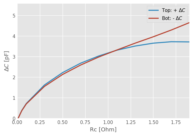
Displayed differently, the distance between capacitances (Top - Bottom) versus coupling resistance is:

delta_C_pos =  np.array(C_matchs)[:,0] - C_matchs[0][0]
delta_C_neg =  C_matchs[0][1] - np.array(C_matchs)[:,1]

fig, ax = plt.subplots()
ax.plot(Rcs, delta_C_pos, label='Top: + $\Delta C$', lw=2)
ax.plot(Rcs, delta_C_neg, label='Bot: - $\Delta C$', lw=2)
ax.set_xlabel('Rc [Ohm]')
ax.set_ylabel('$\Delta C$ [pF]')
ax.set_ylim(bottom=0)
ax.set_xlim(left=0)
ax.legend()

<>:5: SyntaxWarning: invalid escape sequence '\D'
<>:6: SyntaxWarning: invalid escape sequence '\D'
<>:8: SyntaxWarning: invalid escape sequence '\D'
<>:5: SyntaxWarning: invalid escape sequence '\D'
<>:6: SyntaxWarning: invalid escape sequence '\D'
<>:8: SyntaxWarning: invalid escape sequence '\D'
/tmp/ipykernel_2110/2332364399.py:5: SyntaxWarning: invalid escape sequence '\D'
  ax.plot(Rcs, delta_C_pos, label='Top: + $\Delta C$', lw=2)
/tmp/ipykernel_2110/2332364399.py:6: SyntaxWarning: invalid escape sequence '\D'
  ax.plot(Rcs, delta_C_neg, label='Bot: - $\Delta C$', lw=2)
/tmp/ipykernel_2110/2332364399.py:8: SyntaxWarning: invalid escape sequence '\D'
  ax.set_ylabel('$\Delta C$ [pF]')

<matplotlib.legend.Legend at 0x732c1b216a50>

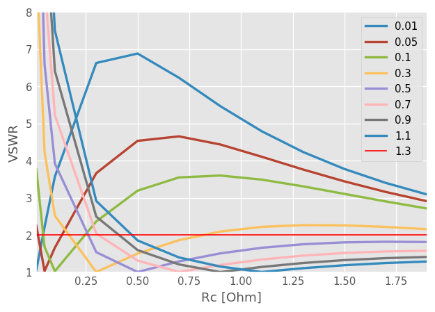
Load Resilience Curves

Ideal loads is usefull to study the behaviour of the load tolerance property of the antenna and the capacitance match points. It is only necessary to work on half-antenna here, because there is no coupling between toroidal elements.

Now that we have figured out the match points, let’s vary the coupling resistances for a fixed match point and look to the return power (or VSWR): this will highlight the load resilience property of the antenna.

# create a single frequency point antenna to speed-up calculations
ant = WestIcrhAntenna(frequency=rf.Frequency.from_f(f_match, unit='Hz'))

fig, ax = plt.subplots()
power = [1, 1]
phase = [0, np.pi]

for C_match in tqdm(C_matchs[0:8]):
    SWRs = []
    ant.Cs = [C_match[0], C_match[1], 150, 150]
    for Rc in Rcs:
        ant.load(Rc)
        SWR = ant.circuit().network.s_vswr.squeeze()[0,0]
        SWRs.append(SWR)
    ax.plot(Rcs, np.array(SWRs), lw=2)

ax.set_xlabel('Rc [Ohm]')
ax.set_ylabel('VSWR')
ax.set_ylim(1, 8)
ax.axhline(2, color='r')
ax.legend(np.round(Rcs, 2))

<matplotlib.legend.Legend at 0x732c1e3e4890>

VSWR(C_top, C_bot) plane

A symetrical Resonant Double Loop (RDL) without mutual coupling between top and bottom strap, has two sets of (symmetrical) solutions. Let’s visualize these solution on a \((C_{top}, C_{bot})\) map.

C_top, C_bot = np.meshgrid(np.arange(40, 60, 1), np.arange(40, 60, 1))

Cs_plane = zip(C_top.flatten(), C_bot.flatten(), C_top.flatten(), C_bot.flatten())

power, phase = [1, 1], [0, np.pi]  # dipole
antenna = WestIcrhAntenna(frequency=rf.Frequency(55, 55, npoints=1, unit='MHz'))

# initiate arrays
results = {}
loads = [0.2, .5, 1, 2]
for load in loads:
    results[load] = []

# calculate VSWR for all (C_top, C_bot) and for different loading cases
for Cs in tqdm(Cs_plane):
    for load in loads:
        antenna.load(load)
        _vswr = antenna.vswr_act(power, phase, Cs=Cs)
        results[load].append(_vswr)

# convert data into arrays
for load in loads:
    results[load] = np.array(results[load])

fig, ax = plt.subplots()

#ax.contourf(C_top, C_bot, np.ones_like(C_top), colors='white')
ax.set_facecolor('white')
ax.grid(True, ls='--', color='gray', alpha=0.5)

for idx, load in enumerate(loads[-1::-1]):
    #map = ax.pcolormesh(C_top, C_bot, results[load][:,0].reshape(C_top.shape),
    #                vmin=1, vmax=1.25, shading='gouraud', cmap='Blues_r')

    cs = ax.contourf(C_top, C_bot, results[load][:,0].reshape(C_top.shape),
                    levels=np.arange(1, 2 ,0.1), alpha=0.7)
    #ax.clabel(cs, inline=True, fontsize=7)
fig.colorbar(cs)
ax.plot([40, 59], [40, 59], ls='--', color='k')
ax.axis([40, 60, 40, 60])
ax.axis('tight')
ax.plot(np.array(C_matchs)[:,0], np.array(C_matchs)[:,1], color='red', ls=':')
ax.set_xlabel('$C_{top}$')
ax.set_ylabel('$C_{bot}$')
ax.set_title('VSWR Map')

Text(0.5, 1.0, 'VSWR Map')

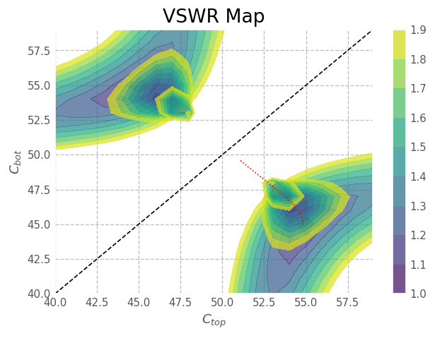
We refer in this package as:

• “Solution 1” the case when \(C_{top} > C_{bot}\)

• “Solution 2” the case when \(C_{top} < C_{bot}\)

from IPython.core.display import HTML
def _set_css_style(css_file_path):
    """
    Read the custom CSS file and load it into Jupyter
    Pass the file path to the CSS file
    """
    styles = open(css_file_path, "r").read()
    s = '<style>%s</style>' % styles
    return HTML(s)

_set_css_style('custom.css')