Plasma Coupling Using COMSOL Results

In this example, we use a COMSOL front-face coupling calculation provided by ORNL, exported as a standard Touchstone file.

The Touchstone file is first import as a scikit-rf Network, which is then modified to fit the WEST ICRH antenna electrical model requirements.

Importing the S-parameters in the electric model

import numpy as np
import skrf as rf

# WEST ICRH Antenna package
import sys; sys.path.append('..')
from west_ic_antenna import WestIcrhAntenna

front_face_conventional = rf.Network(
    '../west_ic_antenna/data/Sparameters/front_faces/COMSOL/ORNL_front_face_conventional.s4p')
print(front_face_conventional)  # 50 Ohm S-param component at a single frequency of 55 MHz

4-Port Network: 'ORNL_front_face_conventional',  55000000.0-55000000.0 Hz, 1 pts, z0=[50.+0.j 50.+0.j 50.+0.j 50.+0.j]

The ports have been defined as: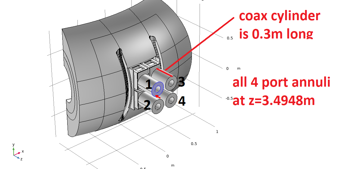

So before to use the S-parameters directly to feed the electrical model, we need to:

• deembed the ports by 0.3m.

• renomalize port reference impedance to the front-face coax characteristic impedances.

• reverse ports 2 and 3 to match the expected definition by the electrical model.

# creating a 50 Ohm dummy coax line to be removed from the front face
media_coax = rf.DefinedGammaZ0(frequency=front_face_conventional.frequency) # 50 Ohm TEM media
extra_line = media_coax.line(d=0.3, unit='m')
# deembed all the 4 ports
for port_idx in range(4):
    front_face_conventional = rf.connect(front_face_conventional, port_idx, extra_line.inv, 0)

/home/docs/checkouts/readthedocs.org/user_builds/west-ic-antenna/checkouts/stable/.venv/lib/python3.12/site-packages/skrf/__init__.py:75: FutureWarning: skrf.io.DefinedGammaZ0 is deprecated. Please import DefinedGammaZ0 from skrf.io.touchstone instead.
  result = getattr(module, name, None)
/tmp/ipykernel_2251/753255592.py:2: FutureWarning: skrf.DefinedGammaZ0 is deprecated. Please import DefinedGammaZ0 from skrf.io instead.
  media_coax = rf.DefinedGammaZ0(frequency=front_face_conventional.frequency) # 50 Ohm TEM media
/tmp/ipykernel_2251/753255592.py:6: FutureWarning: skrf.connect is deprecated. Please import connect from skrf.network instead.
  front_face_conventional = rf.connect(front_face_conventional, port_idx, extra_line.inv, 0)

The COMSOL S-parameters have been exported using a 50 Ohm reference impedance. However, we expect the port reference impedance equals to the characteristic impedance, that is, about 46.64 ohm, so we renormalize the Network to fit this need:

front_face_conventional.renormalize(46.64)  # done inplace

And finally, for historical reasons (may change one day…), the S-matrix port ordering should be adjusted:

front_face_conventional.renumber([1, 2], [2, 1]) # done inplace

OK, so now we can create the WEST antenna object:

ant = WestIcrhAntenna(front_face=front_face_conventional,
                     frequency=front_face_conventional.frequency) # restrict to single frequ

Let’s match the antenna for this coupling:

Cs = ant.match_both_sides(f_match=55e6)

Looking for individual solutions separately for 1st guess...
True solution #1: [52.57985768 45.88696148]
Wrong solution found ! Re-doing...
False solution #1: [150. 150.]
True solution #1: [52.30899414 46.07010622]
Searching for the active match point solution...
Reducing search range to +/- 5pF around individual solutions
True solution #1: [53.67808533 46.12208183 53.62798597 46.30936167]

The coupling resistance of the antenna for this coupling in a nominal dipole excitation is:

power = [1, 1]
phase = [0, np.pi]

# Coupling resistance
ant.Rc(power, phase)

array([0.70081638, 0.6878438 ])

The total voltages and currents at the capacitors are:

power = [1.6/2, 1.6/2]  # MW, to adjust to fit with experiment
phase = [0, np.pi]  # rad

abs(ant.voltages(power, phase))  # results in kV

array([[19.82163699, 21.24743731, 18.39749471, 22.55050911]])

abs(ant.currents(power, phase))  # results in kA

array([[0.62832336, 0.67579437, 0.58405009, 0.71916798]])

Exporting voltage excitations

Now that the electrical model has been created and the antenna matched, one can export the voltage values at the front-face port into COMSOL to visualize the electric field and currents in the antenna front face and in the plasma.

Depending of the needs, the total voltages at the front-face port can be splitted into forward and reflected voltages:

\[V = V_{fwd} + V_{ref}\]

V_fwd, V_ref = ant.front_face_voltage_waves(power, phase, Cs=Cs)
print(V_fwd)

[[ -6.69328078-28.99509562j   5.99357198+27.60123209j
   22.77200553+16.48928635j -22.07805377-14.78481093j]]

Of course, we find the same total voltage:

Vtot = V_fwd + V_ref
V = ant.voltages(power, phase, Cs=Cs)
# pay attention that the voltage index differ from the front-face port indexes...
np.allclose(Vtot[:,[0,2,1,3]], V, rtol=1e-5)

True

It is also possible to deduce the forward powers and phases to setup on the four ports (assuming the reference impedance is real):

powers, phases = ant.front_face_powers_phases(power, phase, Cs=Cs)
print(powers) # in Watt
print(phases) # in degrees

[[9.49309153 8.55221824 8.47406518 7.56894396]]
[[-102.99856575   77.74849927   35.90842469 -146.19132356]]